Na primeira vez que você se prepara para baixar um grande modelo, as indicações 7B, 32B, 128K e INT4 na página do modelo podem ser confusas: 7B indica o tamanho do modelo, 128K soa como se pudesse conter um livro inteiro, e INT4 pode reduzir o uso de VRAM. Como isso funciona?
Depois de começar a usar modelos na prática, você encontrará problemas adicionais: atas de reunião que não cabem, conversas longas onde o contexto anterior é esquecido, respostas do modelo sem fundamentação, e o mesmo modelo se comportando de forma diferente com diferentes métodos de quantização.
Para determinar se um modelo é adequado para uma tarefa específica, você precisa entender como o texto entra no modelo, como as capacidades do modelo são treinadas e por que o modelo consome memória e VRAM durante a inferência.
Este conhecimento pode ser organizado ao longo de três linhas principais. The first starts with the overall Transformer architecture, then covers Tokens, Embedding, and Attention to explain how a piece of text enters and is processed by the model. The second covers pre-training, instruction fine-tuning, and post-training to explain how model capabilities are formed. The third covers context length, KV Cache, quantization, and hardware, which determine whether a model can run stably on target devices.
This chapter distills foundational knowledge from earlier related chapters. For model inference, you can refer to Chapters 6 and 7. For model SFT, you can refer to Chapter 9's introduction to the built-in ms-swift fine-tuning framework. For post-training content, you can also refer to Chapter 10's coverage of preference alignment and reinforcement learning. For domain model applications and hallucination issues, you can also refer to Chapter 13's introduction to RAG methods, which use external knowledge to improve domain-specific QA and further reduce model hallucinations.
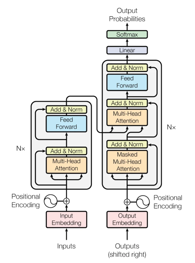
O Transformer é a arquitetura fundamental utilizada pela maioria dos grandes modelos de linguagem atuais. Unlike earlier recurrent neural networks that process text sequentially, Transformer can compute multiple positions in parallel during training and input processing, and establishes connections between different positions through Attention. A classic Transformer consists of an Encoder and a Decoder. Each Transformer layer typically contains Attention and a Feed-Forward Network. The feed-forward network, also called FFN or MLP, applies nonlinear transformations to the vectors at each position. Residual connections and layer normalization are also used within layers to help information flow stably through deep networks. When many similar layers are stacked, the model gradually develops complex text representation and generation capabilities. The overall Transformer architecture is shown in the figure below: the left side is the Encoder and the right side is the Decoder. The N× in the figure indicates that similar modules are stacked multiple times; the actual number of layers varies depending on the model architecture and parameter scale.
Entrar participar da discussão
During model inference, when a user inputs a piece of text, the model undergoes the following processing: first, the Tokenizer splits the raw text into individual Tokens and converts them into corresponding Token IDs. Then, the Embedding layer maps these discrete Token IDs into continuous vector representations, while adding positional information so the model knows the order of each Token in the sentence. Next, these vectors pass through multiple Transformer layers for repeated processing, where the Attention mechanism allows different Tokens to attend to each other and exchange contextual information, and the feed-forward network further processes the features at each position. After multiple layers of computation, the model obtains a comprehensive representation of the current context, calculates the probability distribution for the next Token, selects or samples the next Token, and adds it to the context to repeat this process until the entire content is generated.
The three components in the original Transformer each serve different purposes:
- Encoder-only structure: Primarily responsible for understanding input; it can simultaneously reference different positions in the input sequence, suitable for tasks such as classification, extraction, and semantic representation;
- Decoder-only structure: Primarily responsible for generating output; when generating the current position, it can only view content that has already appeared;
- Encoder-Decoder structure: First understands input, then gradually generates output, commonly used in sequence-to-sequence tasks such as translation and summarization.
Modern large models don't necessarily use complete Encoder and Decoder simultaneously. On this foundation, various architectures derived from Transformer have emerged. For example, GPT-type generative models typically use Decoder-only structure, BERT-type models mainly use Encoder-only, and T5-type models retain the Encoder-Decoder structure.
A Token is the basic unit used when the model reads and generates text. It can be a Chinese character, a word, part of a word, punctuation, or even whitespace or special control markers. For example, the same sentence may produce different results with different Tokenizers:
Original: Large language models are changing the way offices work.

Tokenizer A: Large / language / models / are / changing / office / ways / .
Tokenizer B: Large / language / models / are / chang / ing / office / ways / .
Both results express the same sentence, but the number of Tokens differs. What the model actually receives is the numeric ID corresponding to each Token, known as the Token ID. Using meeting minutes as an example, what the model sees isn't a complete meeting record but a sequence of Token IDs. The meeting name, spoken content, time, punctuation, and output requirements all consume Tokens; the summary, conclusions, and action items generated by the model also continue to consume Tokens. Therefore, the more detailed the output required from the same material, the less space remains for the original record.
If tokens are split entirely by character, the vocabulary can be relatively small but sequences become longer. If split entirely by complete words, the vocabulary becomes very large and will constantly encounter new words, abbreviations, and spelling variations. Large models typically use subword tokenization, finding a balance between characters and complete words. BPE, WordPiece, Unigram, and SentencePiece are all common methods.
Usually, the model cannot directly perform matrix operations on text or images; it first needs to convert content into numerical vectors. This process is called Embedding or vector representation. For text, the Tokenizer first converts the text into Token IDs, and the Embedding layer then looks up the corresponding vectors based on the IDs. A single number in a vector usually has no intuitive meaning, but the entire vector can represent the features of that Token within the model. Taking the Token "meeting" as an example, the corresponding Token ID might be a specific integer such as "15872", and the representation of that Token, i.e., its Embedding, could be a vector like [0.12, -0.37, 0.08, ...]. Embeddings are continuously adjusted during training, and Tokens that appear in similar contexts tend to form similar features in their vectors. Due to differences in model architecture and training, the same word processed through multiple Transformer layers will also form different representations based on context.
When the model acquires semantic information from input text, it needs to know not only what the Token is, but also where it is located. With Token Embedding alone, for example, "meeting postponed" and "postponed meeting" contain similar Tokens but express different meanings due to word order differences. Therefore, the model also needs positional encoding or positional representation. The figure below uses BERT's input layer as an example.
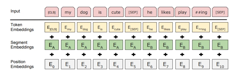
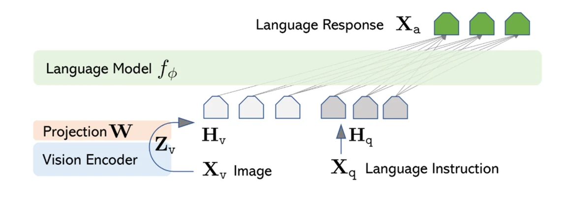
As shown in the representation method used in BERT above, the figure demonstrates the combination of Token Embedding, Segment Embedding, and Position Embedding. Of course, different model architectures and design approaches use different specific methods. For multimodal large models, images, audio, and other content also need to be converted into vectors first. Images are typically divided into patches, with visual encoders extracting features; audio is first converted into acoustic features, then processed by audio encoders. Features from different modalities must pass through a Projection module before entering the vector space that the large model can process. As shown in the figure below, the Projection module fuses image information with semantic information.
Attention determines which parts of the input the current position should focus on. It computes relevance based on the model's existing vector representations, rather than just matching identical words. For example, in the sentence "The project was delayed, and the report explained why it wasn't completed on time," when the model processes the pronoun "it," it needs to combine context to determine whether it more likely refers to "project" or "report." When extracting responsible persons from meeting records, the model also needs to connect task descriptions, personnel names, and sentences indicating division of labor.
Each input vector undergoes different transformations to form Query, Key, and Value, commonly abbreviated as Q, K, and V. The Attention formula can be simplified as:
$\mathrm{Attention}(Q, K, V)=\mathrm{softmax}\left(\frac{QK^{\mathrm{T}}}{\sqrt{d_k}}\right)V$
Here, Q represents what information the current position is looking for, K represents what features each position can be matched by, and V represents the content to be retrieved after matching. The model first compares Q and K to obtain relevance scores between the current position and other positions, then converts scores to weights through softmax, and performs weighted aggregation of V according to the weights. The $d_k$ in the formula is the dimension of the Key vector; dividing by $\sqrt{d_k}$ adjusts the score scale to make computation more stable.
If Q, K, V all come from the same sequence, it is called Self-Attention, used to establish connections within a sequence. If Q comes from one sequence while K and V come from another, it is called Cross-Attention. For example, an Encoder-Decoder translation model can allow the Decoder to read source text information from the Encoder through Cross-Attention.
For generative large models, the current position can only reference content that has already appeared, so Attention must include a causal mask to block subsequent positions. Even with future Tokens masked, the number of relationships processed by full causal attention still grows approximately quadratically with sequence length. During the generation phase, historical Token K and V must also be stored, forming the KV Cache described later. As context grows longer, Attention computation and cache overhead become increasingly prominent. The different structures introduced below evolved specifically to address these issues.
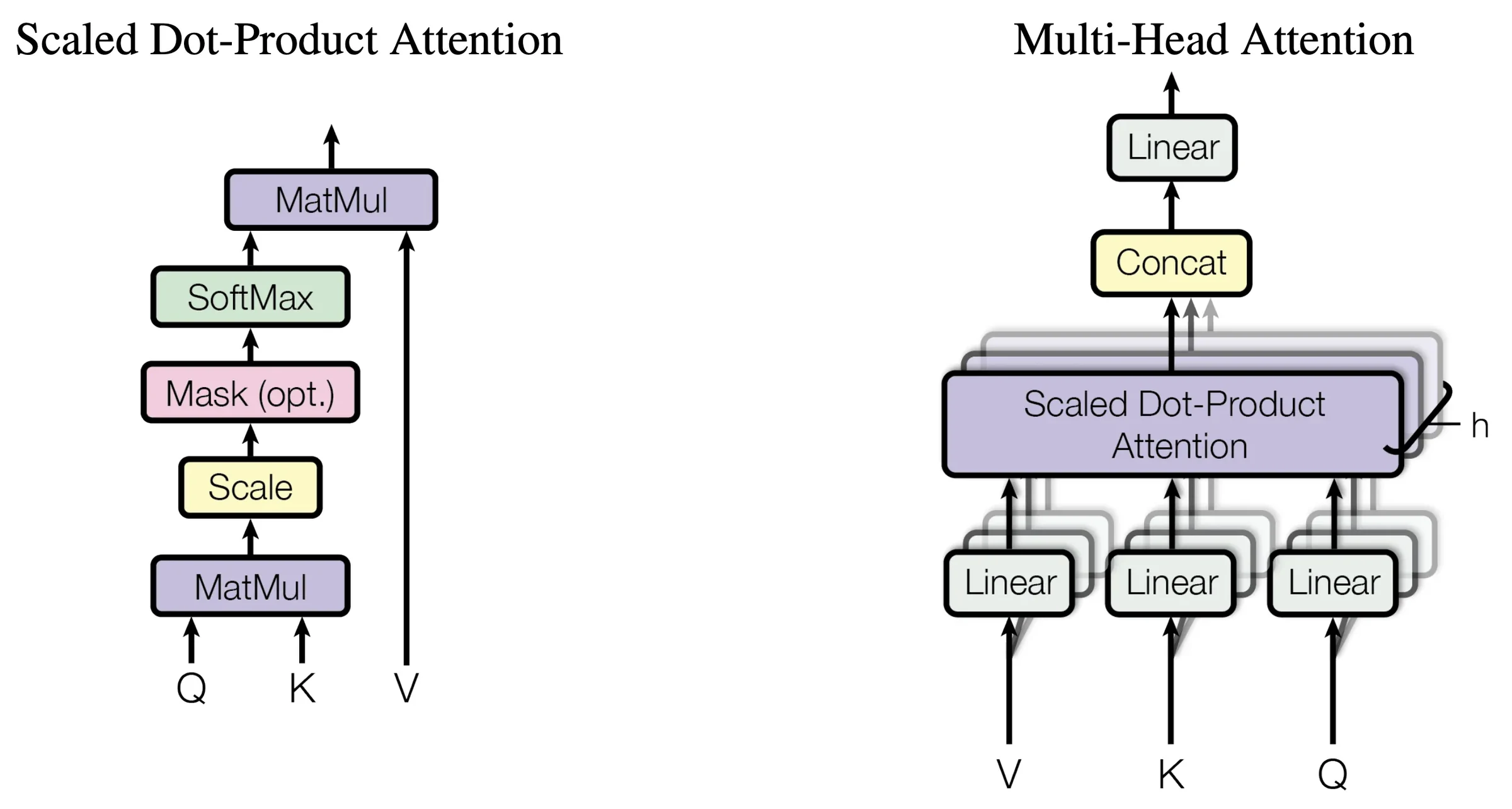
Multi-Head Attention (MHA) was proposed in the 2017 Transformer paper "Attention Is All You Need" and later applied to BERT and models like Llama 2 7B and 13B. It adds multiple parallel attention heads on top of a single set of attention computations, enabling the model to extract contextual relationships from different representation spaces.
In MHA, each head has its own projection parameters for generating Q, K, and V, computes attention separately, and then concatenates the results from all heads and passes them through a linear layer to form the output. As shown in the figure below, the left side shows the computation process for one set of scaled dot-product attention, while the right side runs this process multiple times in parallel and then fuses the results. The focus patterns of different heads are formed during training and can jointly support tasks such as coreference resolution, semantic association, and long-distance dependency.
MHA improves the model's ability to aggregate different types of information and facilitates parallel computation during training. However, during token-by-token generation, each head must read its own historical K and V. As the number of model layers, heads, and context length increases, this cache and data reading consumes significant resources. Therefore, subsequent improvements first considered whether multiple Query heads could be retained while reducing the number of Key heads and Value heads that need to be stored.
Multi-Query Attention (MQA) was proposed by Noam Shazeer in the 2019 paper "Fast Transformer Decoding: One Write-Head is All You Need" and later applied to large models like Falcon-7B. It primarily addresses the memory bandwidth problem during decoding: when the model generates each new Token, it needs to read the existing KV Cache. When the read volume is too large, generation speed is limited even if the compute units still have capacity.
MQA retains multiple Query heads but lets them share a single set of Key and Value. This way, different heads can still generate different queries, but historical positions only need to store one copy of K and V for all heads to share. The figure below shows one initialization method for converting an existing MHA model to MQA: averaging multiple Key projection matrices to obtain a shared projection, with Value projection treated the same way. After conversion, further training is needed to adapt the model to the new shared structure.
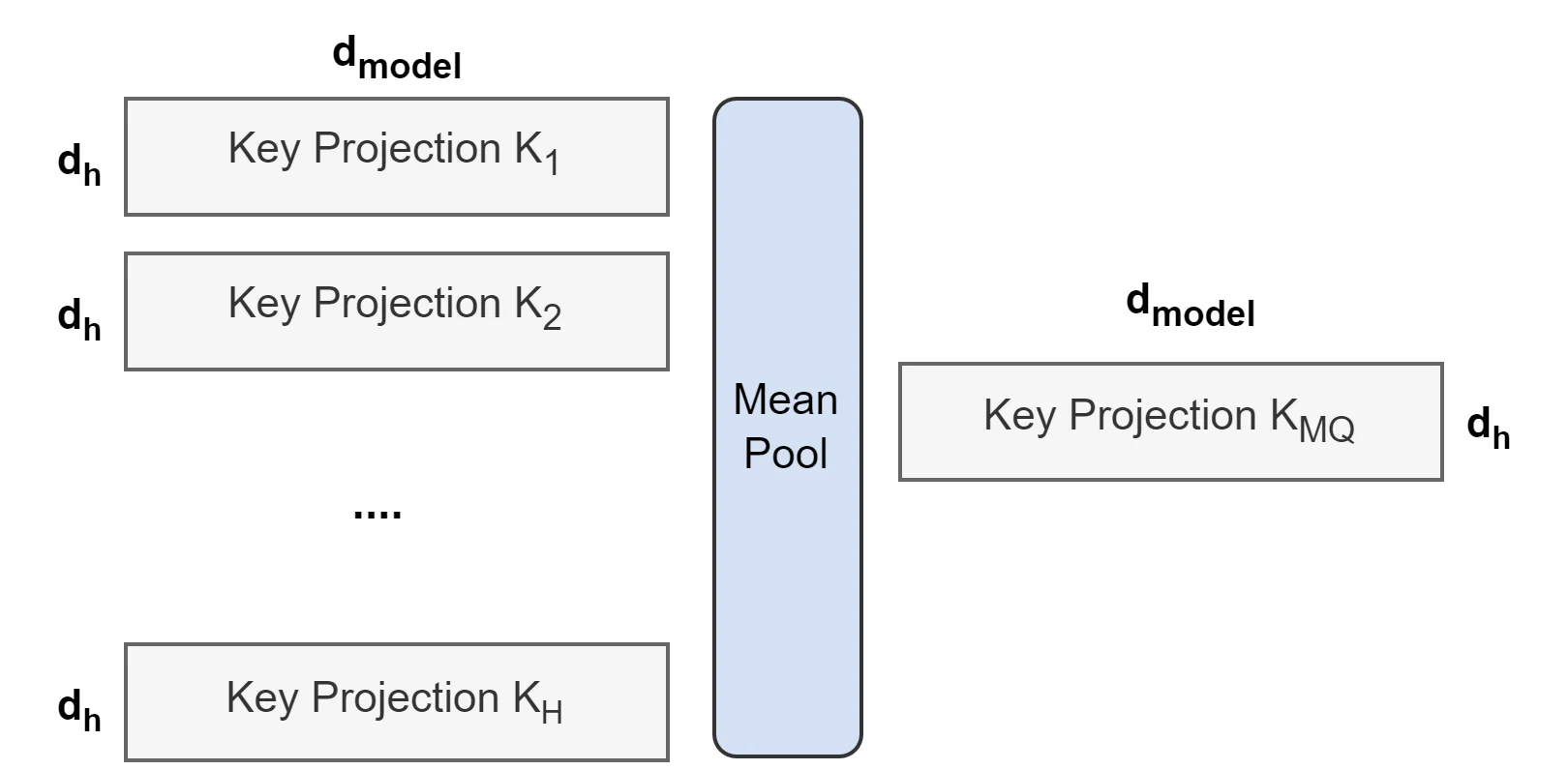
With this structure, MQA can significantly reduce KV Cache and the data reading volume per decoding step, freeing up space for longer inputs or more concurrent requests. For example, Falcon-7B is configured with 71 Query heads but only 1 KV head. Compared to a 71-group KV structure with the same head dimension and precision, its theoretical KV cache is only about 1/71. However, sharing also constrains the representation capacity of K and V, so training and evaluation are needed to confirm the impact of this efficiency gain on task quality.
Grouped-Query Attention (GQA) was systematically proposed by the Google Research team in the 2023 GQA paper and applied to large models like Llama 2 70B and Mistral 7B. It aims to balance the multi-group representation capability of MHA with the low cache overhead of MQA, avoiding the situation where all Query heads must use the same set of K and V.
GQA divides Query heads into several groups, with each group sharing a single set of Key and Value, while different groups retain different K and V representations. As shown in the figure below, MHA configures a corresponding set of K and V for each Query head, MQA lets all Query heads share one set of K and V, and GQA shares within groups. When the number of groups equals the number of Query heads, GQA is equivalent to MHA; when there is only one group, it is equivalent to MQA.
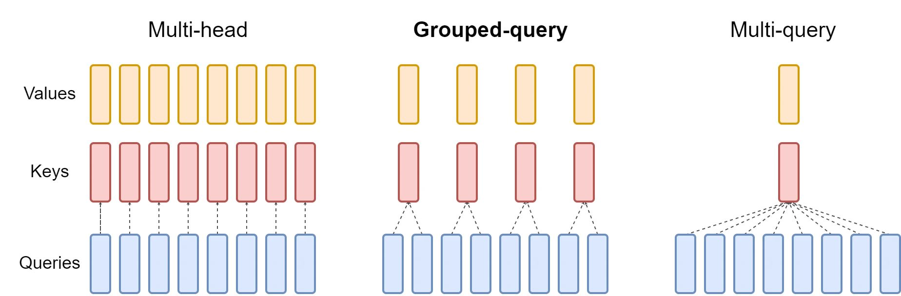
Taking Mistral 7B v0.1 as an example, it has 32 Query heads and 8 KV heads, with every 4 Query heads sharing one set of K and V. With the same head dimension and precision, this cache is approximately 1/4 that of MHA. For practical deployment, reducing cache and reading volume generally helps improve concurrency and decoding efficiency. Since different groups still retain their own K and V, GQA also retains more representation space than fully shared MQA. What is reduced here is the number of KV heads; the model can still compute attention for all historical positions it is allowed to access.
Sliding Window Attention (SWA) comes from the local attention approach in long sequence modeling. Mistral 7B v0.1 uses it in combination with GQA. GQA reduces the number of KV heads that need to be stored per position, while SWA further limits the historical range that each position directly attends to, reducing computation and cache pressure for long texts.
SWA sets a fixed-size window for each Token, computing attention only for recent positions within the window. The figure below shows complete causal attention on the left, Sliding Window Attention in the middle, and on the right, how information passes backward through multiple network layers. Although a single layer only reads the local range, the Token representation from the previous layer already contains earlier contextual information, so after processing through multiple layers, the model can indirectly utilize content beyond the window.
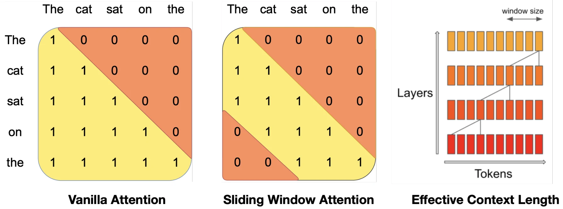
Mistral 7B v0.1 uses a window of 4096 Tokens and employs a rolling cache to cover old K and V that have moved out of the window, allowing each layer's cache to be maintained within a fixed range. In the paper's tests with 16K sequence length and 4096 window, with corresponding kernel optimization, speed was approximately 2x that of the full attention baseline. This structure can control resource growth for long texts, but remote original details must pass through intermediate representations, so the local window size cannot be directly equated with the context length the model can accurately retrieve.
Multi-head Latent Attention (MLA) was proposed by the DeepSeek team in DeepSeek-V2 and subsequently used in DeepSeek-V3. It also addresses the problem of excessive KV Cache but further changes the storage format: by learning a compact joint representation, it reduces the amount of data that needs to be stored per Token while supporting multiple attention heads using this information.
Specifically, MLA first uses low-rank projection to jointly represent K and V as lower-dimensional latent vectors. During inference, only this vector and the Key component that independently carries rotary positional information are cached. Multiple Query heads can use this shared representation for matching and information aggregation, and some projection matrices can be merged during inference, reducing the need to explicitly expand complete K and V. The hatched areas in the figure below indicate the content that needs to be cached, showing how MLA transfers the multi-head K and V cache to the smaller latent representation on the right.
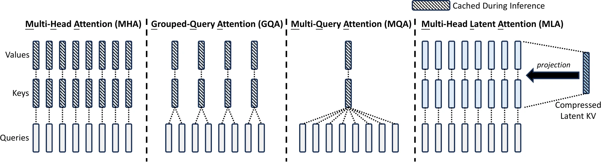
This design enables DeepSeek-V2 and V3 to maintain multi-head expressive capability while reducing cache pressure during long-context generation. In the DeepSeek-V2 report, MLA's per-Token KV cache size is equivalent to only 2.25 groups of KV heads in GQA. It compresses the representation dimension at each position; historical positions themselves are still retained, so in full attention mode, the model still needs to read and match all historical entries. To further reduce the number of entries participating in computation each time, sparse attention must be introduced.
DeepSeek Sparse Attention (DSA) was proposed by the DeepSeek team and applied to DeepSeek-V3.2-Exp and DeepSeek-V3.2. Building on MLA, it adds a dynamic selection mechanism to address the problem where, even when individual KV entries are already small, reading and computing all historical entries in long contexts is still expensive.
DSA first uses a lightweight indexer called Lightning Indexer to compute relevance scores between the current Query and historical Tokens, then selects the Top-k positions with the highest scores for the main Attention to process. The green area in the figure below is the new indexing process, where the Top-k Selector chooses positions, and the core Attention above reads the MLA cache corresponding to the selected positions. The indexer uses smaller representations and fewer heads to complete filtering, with computation costs lower than directly executing the full main Attention.
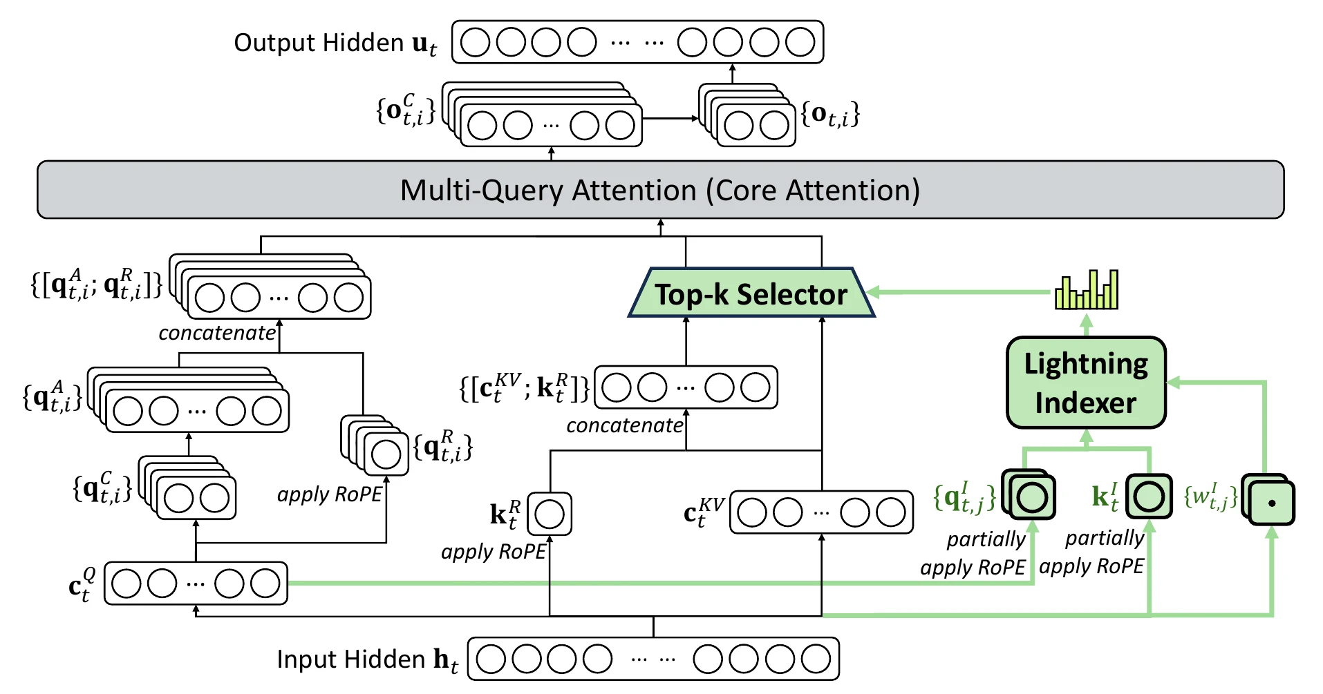
In the DeepSeek-V3.2 report, the configuration is that each Query can select up to 2048 KV entries. As context grows, the core Attention can still focus on this limited range, significantly reducing the cost of long input processing and subsequent generation. Historical entries not selected in this round are still available for subsequent Queries to retrieve, so sparse selection primarily reduces the reading and computation volume this time, rather than removing all cache in the same proportion. The indexer itself still needs to process historical candidates, and actual overhead is also affected by context length.
MiniMax Sparse Attention (MSA) was proposed by the MiniMax team and applied to MiniMax-M3. It addresses efficiency issues in million-Token contexts, particularly considering how to make sparse attention suitable for GPU batch computation, rather than just theoretically reducing the number of Tokens participating in computation.
MSA builds on GQA and includes an indexing branch and a main branch. The indexing branch first computes Token-level relevance scores, then takes the highest score within each block as the block score, selecting Top-k historical blocks for different GQA groups separately. The main branch then reads Token-level K and V from the selected blocks that satisfy causal conditions, while retaining the current local block. As shown in the figure below, the two Query groups on the right can form different selection ranges, while Query heads within the same group share selection results.
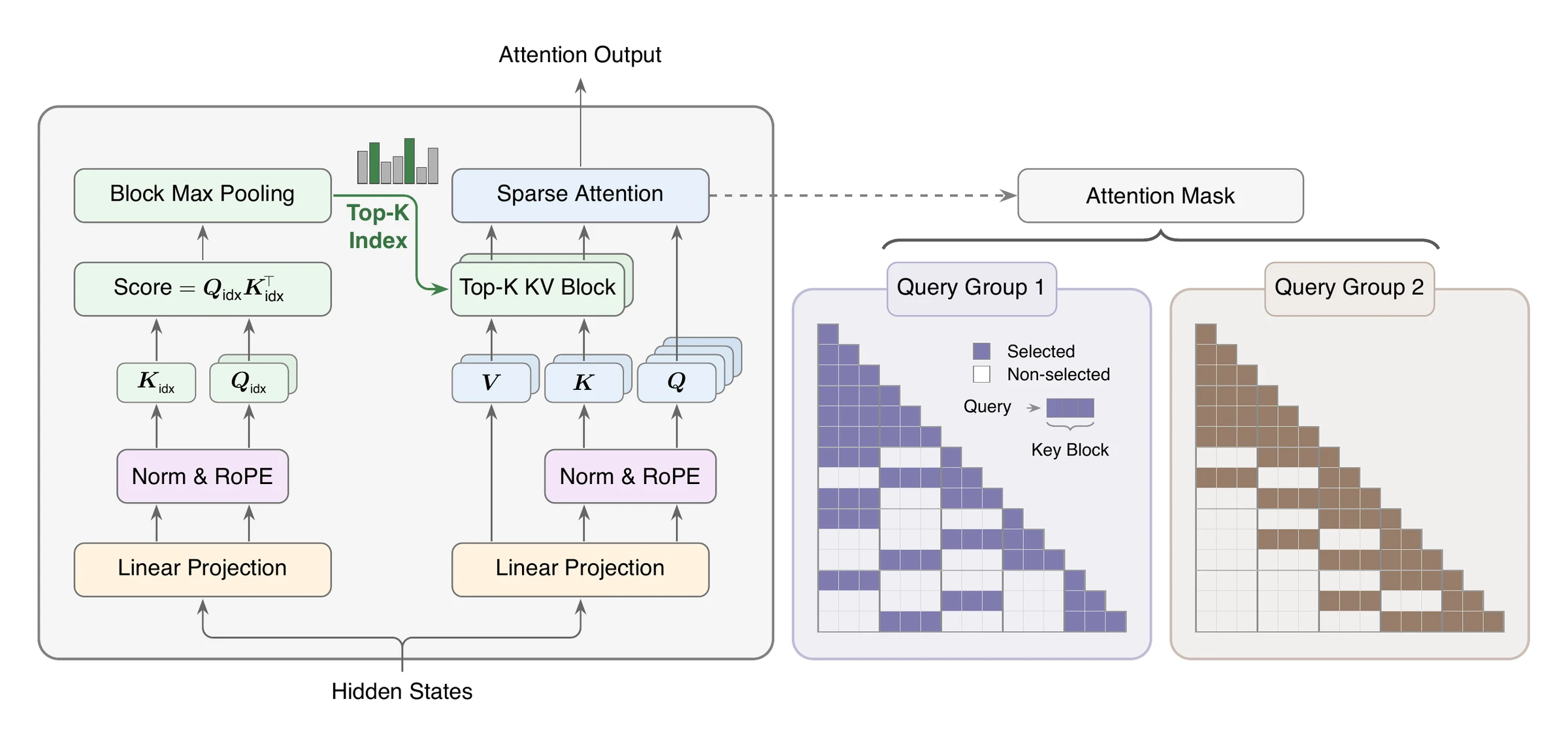
Organizing access by blocks improves the regularity of GPU data processing, and grouped selection allows different groups to retain different retrieval patterns. In the 1M context test of the 109B parameter experimental model, the paper reports that MSA's per-Token attention computation is approximately 1/28.4 of GQA. With specialized kernels, the Prefill phase for processing input and the Decode phase for token-by-token generation on H800 achieved approximately 14.2x and 7.6x speed improvements respectively. This demonstrates that sparse algorithms and compute kernels must be co-designed; reducing computation volume can only be fully converted into actual speed benefits through such joint optimization.
Qwen Sparse Attention (QSA) was proposed by the Qwen team and applied to Qwen3.8-Flash-Next. This model uses a hybrid structure of three layers of Gated DeltaNet combined with one layer of QSA: the former efficiently processes sequences through state updates, while the latter retains direct retrieval of historical Tokens. The key problem QSA addresses is that indexers themselves generate significant overhead in long contexts.
To this end, QSA first compresses the indexing Keys of consecutive Tokens into micro-block representations through average pooling, computes relevance scores on the shorter micro-block sequence, and selects Top-k blocks. After selection, it expands blocks back to original Token positions, allowing the core Attention to read the corresponding K and V. Tail Tokens that haven't formed complete blocks are also retained. The left side of the figure below shows the compressed indexing process, and the right side shows the micro-block sparse Attention based on selection results, with position indices passed between the two parts.
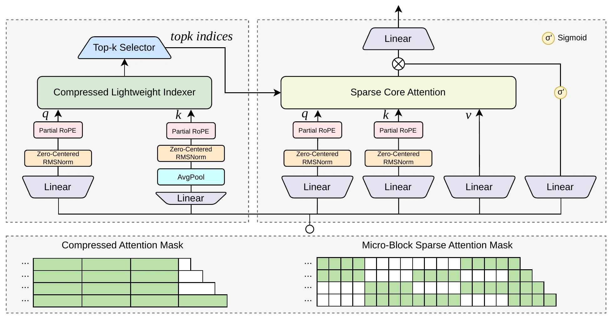
This both reduces the positions the main Attention accesses and shortens the sequence the indexer needs to scan. The Qwen3.8-Flash-Next report shows that in kernel tests with 1M context, QSA achieved approximately 7.6x and 4.9x speed improvements in Prefill and Decode respectively compared to dense attention. When understanding this structure, it is important to distinguish between the index representation and the main Attention cache: QSA compresses the former to reduce filtering costs, but after selection still reads Token-level KV, so fine-grained information in the selected region can be preserved.
Kimi Delta Attention (KDA) was proposed by the Moonshot AI team in Kimi Linear and is practically applied in the Kimi Linear model with 48B total parameters and 3B activated parameters. It adopts a linear attention approach, continuously writing historical information into a fixed-size state, reducing the overhead of repeatedly reading long historical sequences at each generation step.
KDA builds on Gated DeltaNet and introduces finer-grained gating. When a new Token arrives, the model first controls the degree of information retention for different channels in the old state, then corrects existing key-value associations through the Delta rule. This update can be understood as using the difference between the new input and the content predicted by the current state to adjust the information stored in the state. Since the decay gate varies by channel, different parts can use different retention rates. During computation, blocks of Tokens can also be processed in parallel to improve GPU efficiency.
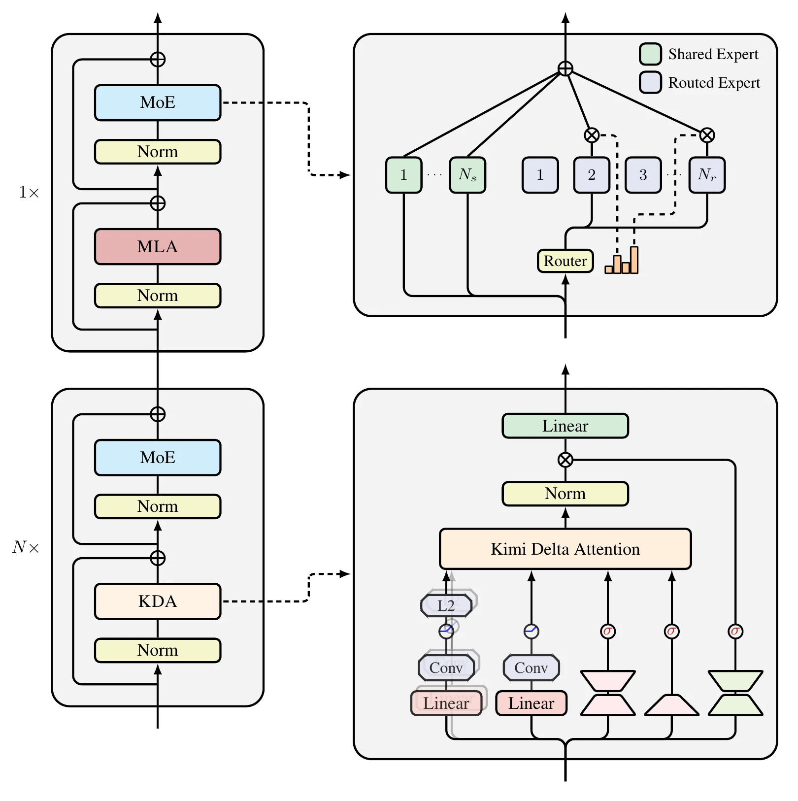
The figure above shows how Kimi Linear interleaves three layers of KDA with one layer of MLA. The KDA layer uses fixed-size state to reduce long sequence costs, while the MLA layer supplements direct retrieval of specific historical positions, alleviating the limited capacity of fixed state. In comparisons using the same training scheme, this hybrid model reduced KV Cache by up to 75% compared to the full MLA baseline and achieved up to approximately 6x decoding throughput at 1M context. These results correspond to Kimi Linear's hybrid architecture rather than being a uniform configuration across all Kimi models.
Compressed Sparse Attention (CSA) was proposed by the DeepSeek team in DeepSeek-V4 and applied to DeepSeek-V4-Pro and DeepSeek-V4-Flash. While the earlier MLA primarily compresses the KV representation of each Token, CSA further reduces the number of entries along the sequence dimension, aggregating information from multiple Tokens into fewer KV entries, then performing sparse selection.
CSA first processes consecutive Tokens with a learnable Token-level compressor, combining overlapping information from adjacent blocks to form compressed KV. Then, Lightning Indexer scores these compressed entries and selects Top-k entries for the main Attention. In the figure below, the compressor is positioned before indexing and selection, and the main Attention directly reads the compressed KV. On the left, a sliding window branch also sends recent uncompressed Tokens into the computation, preserving local details.
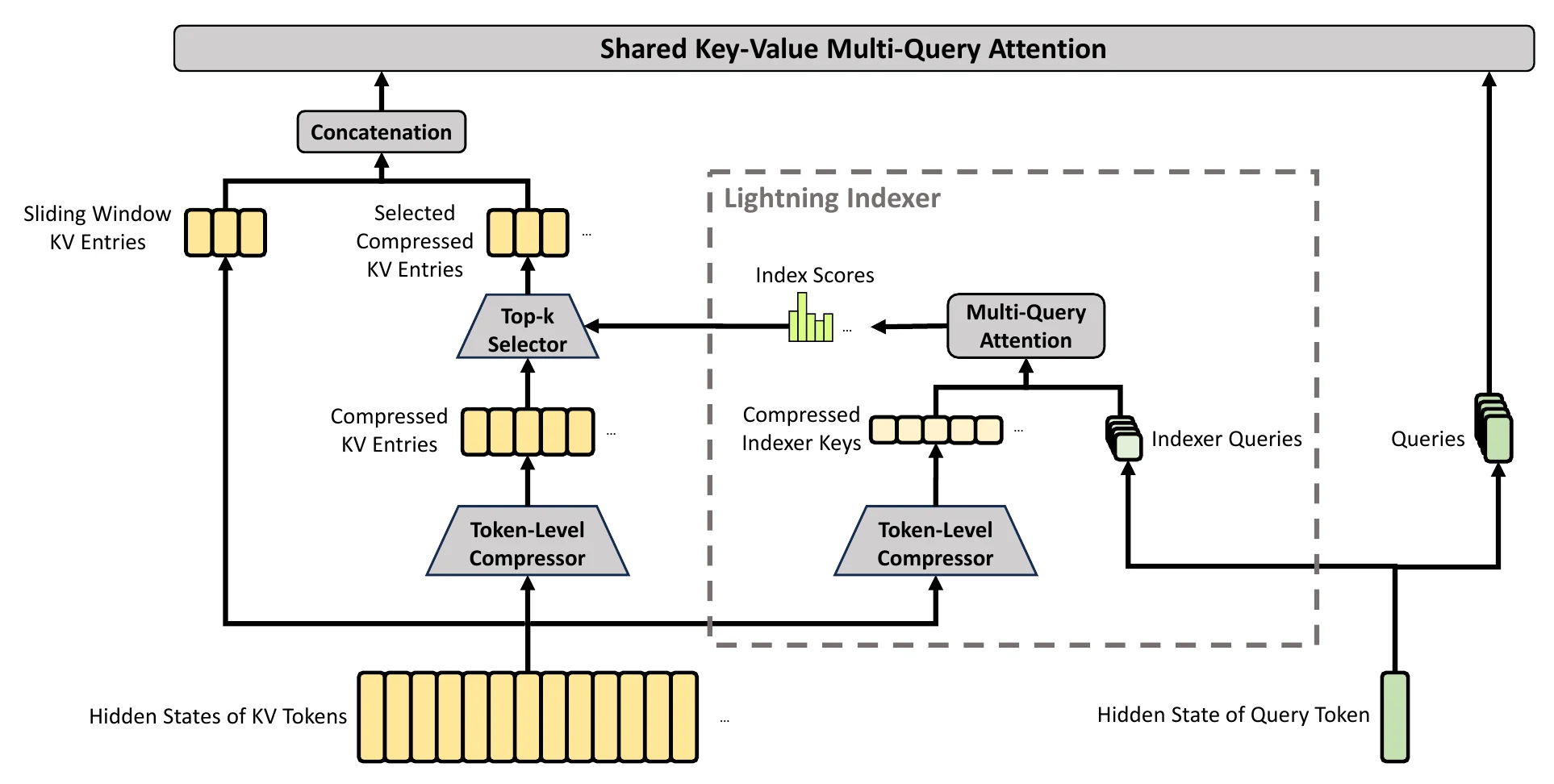
In the DeepSeek-V4 report, CSA has a compression ratio of 4, meaning historical KV entries are reduced to approximately one-quarter, with a subset selected for core Attention computation. Thus, CSA both reduces long-term cache volume and decreases the historical content read and computed each time. QSA compresses the index but then returns to original Tokens, while CSA directly completes information aggregation on compressed entries, thus also compressing the historical KV itself. This design requires the compressor to preserve useful features, supplemented by the local window for recent details.
Heavily Compressed Attention (HCA) was also proposed by the DeepSeek team in DeepSeek-V4 and is used in alternation with CSA in the multi-layer structure of DeepSeek-V4-Pro and Flash. It employs stronger sequence compression, allowing the model to retain coverage of large-scale historical information with less cache, complementing CSA's selective reading.
HCA's compression ratio is set to 128 in the report, far higher than CSA's 4. After multiple Tokens are aggregated into a single compressed entry through learnable weighted summation, the current Query performs Attention on all causally visible compressed history without Top-k selection. As shown in the figure below, HCA retains the compressed branch and local sliding window branch but omits the indexer and selector from CSA. The window provides recent Token details, while the compressed history provides broader contextual information.
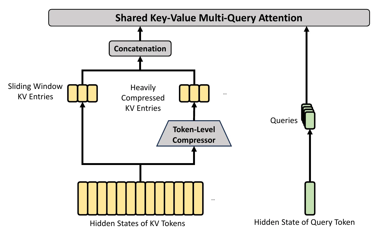
The alternating configuration of CSA and HCA enables DeepSeek-V4 to simultaneously utilize historical representations at different granularities. According to the report, at 1M context, DeepSeek-V4-Pro's single-Token inference FLOPs and KV Cache are approximately 27% and 10% of DeepSeek-V3.2's respectively. This is the combined effect of the hybrid Attention structure along with low-precision computation and storage. For users, the significance of this type of structure is that it makes ultra-long contexts easier to run on limited hardware. Whether a specific model can accurately extract details from long materials still depends on the compression method, training process, and actual task.
From these model designs, we can see that Attention improvements are not limited to a single direction. MHA, MQA, and GQA primarily change the sharing relationship between heads; MLA compresses the KV representation at each position; DSA, MSA, and QSA reduce the positions accessed by the core Attention; KDA processes history through state updates; and CSA and HCA further compress historical entries. Models can combine multiple of these methods, so when analyzing resource requirements, it is necessary to consider the number of layers and cache format for each structure. Regardless of which structure is used, Attention is only responsible for aggregating contextual information; the model's overall capability is jointly formed by Attention together with Embedding, the feed-forward network, and the training process.
Model architecture determines how information is computed, while the training process determines what the model ultimately learns. Large model training is typically divided into several stages. First, in the pre-training stage, the model learns language patterns, knowledge structures, and basic reasoning patterns from massive text, code, and other data, gaining general capabilities. Next, it enters the Instruction Fine-Tuning (SFT) stage, where through large numbers of "instruction-response" examples, the model learns to understand user requirements and respond in the specified task format. On this basis, further preference optimization or reinforcement learning is performed, adjusting model behavior based on human feedback or rules to make responses better align with expectations in terms of usefulness, accuracy, expression style, safety, and behavioral boundaries.
Pre-training is the stage where the model forms its foundational capabilities. The model is trained repeatedly on large-scale text, code, or multimodal data. For Decoder-only language models (such as the GPT series), the common training task is to predict the next Token based on preceding content, adjusting model parameters when predictions are wrong. After massive samples are repeatedly processed, the model gradually learns language structure, expression patterns, and statistical relationships between different concepts, and develops the foundational representation and generation capabilities needed for tasks such as question answering, summarization, translation, and code generation.
The knowledge acquired during pre-training is distributed across a vast number of parameters, not a database that can be queried item by item. The model can combine learned patterns to generate content that doesn't appear verbatim in training data, and may also combine related but not fully matching information to form seemingly plausible but incorrect answers. Of course, more training data is not always better. Repeated content, low-quality web pages, incorrect knowledge, privacy data, and harmful content all affect the model. Before pre-training, format parsing, deduplication, quality filtering, safety filtering, and data proportioning are typically required. Data scale determines how much content the model can access, while data quality directly affects what the model can learn from it.
After completing pre-training, the model can already continue text, but it doesn't necessarily reliably complete tasks according to user requirements. For example, if the user asks to list three action items, the base model might continue expanding the question or ignore the specified format. Instruction fine-tuning uses examples consisting of instructions and expected answers to continue training the model. Here is an example of instruction fine-tuning:
Instruction: Organize the following meeting minutes into action items.
Input: Meeting minutes text.
Output: A table containing tasks, responsible persons, and deadlines.
Through training on different types of examples including Q&A, summarization, information extraction, code, tool calling, and safety refusal, the model gradually learns to recognize user intent and follow output requirements. Instruction fine-tuning primarily teaches the model how to use its existing capabilities. It can supplement some knowledge but is not suitable for solving all knowledge update problems. Content that requires frequent updates or must provide sources is better served through knowledge bases, retrieval, or external tools at runtime.
Post-training is the collective term for a series of training and alignment work performed after the model completes pre-training. Instruction fine-tuning is typically part of post-training, and further instruction fine-tuning (SFT), preference optimization, and reinforcement learning may also appear at this stage. Therefore, instruction fine-tuning and post-training are not two independent steps; the former is a specific method category, while the latter is a stage encompassing multiple methods. Several training approaches can first be understood according to the following relationship:
Stage or Method | Primary Data Used | Primary Problem Addressed |
Pre-training | Large-scale text, code, and multimodal data | Teaching the model fundamental patterns like language and knowledge |
Instruction Fine-tuning / SFT | Instructions and expected responses | Teaching the model to output according to task requirements |
Preference Optimization | Better and worse responses to the same question | Making the model prefer responses that align with preferences |
Reinforcement Learning | Prompts, model responses, and reward signals | Continuing to adjust generation strategy based on rewards |
Referring to the Reinforcement Learning from Human Feedback (RLHF) framework used in InstructGPT, a classic post-training pipeline has been established. RLHF typically uses human demonstration data to complete SFT in the first step, uses response ranking data to train a reward model in the second step, and uses PPO to optimize the language model's generation strategy based on scores from the reward model in the third step. The specific process is shown in the figure below.
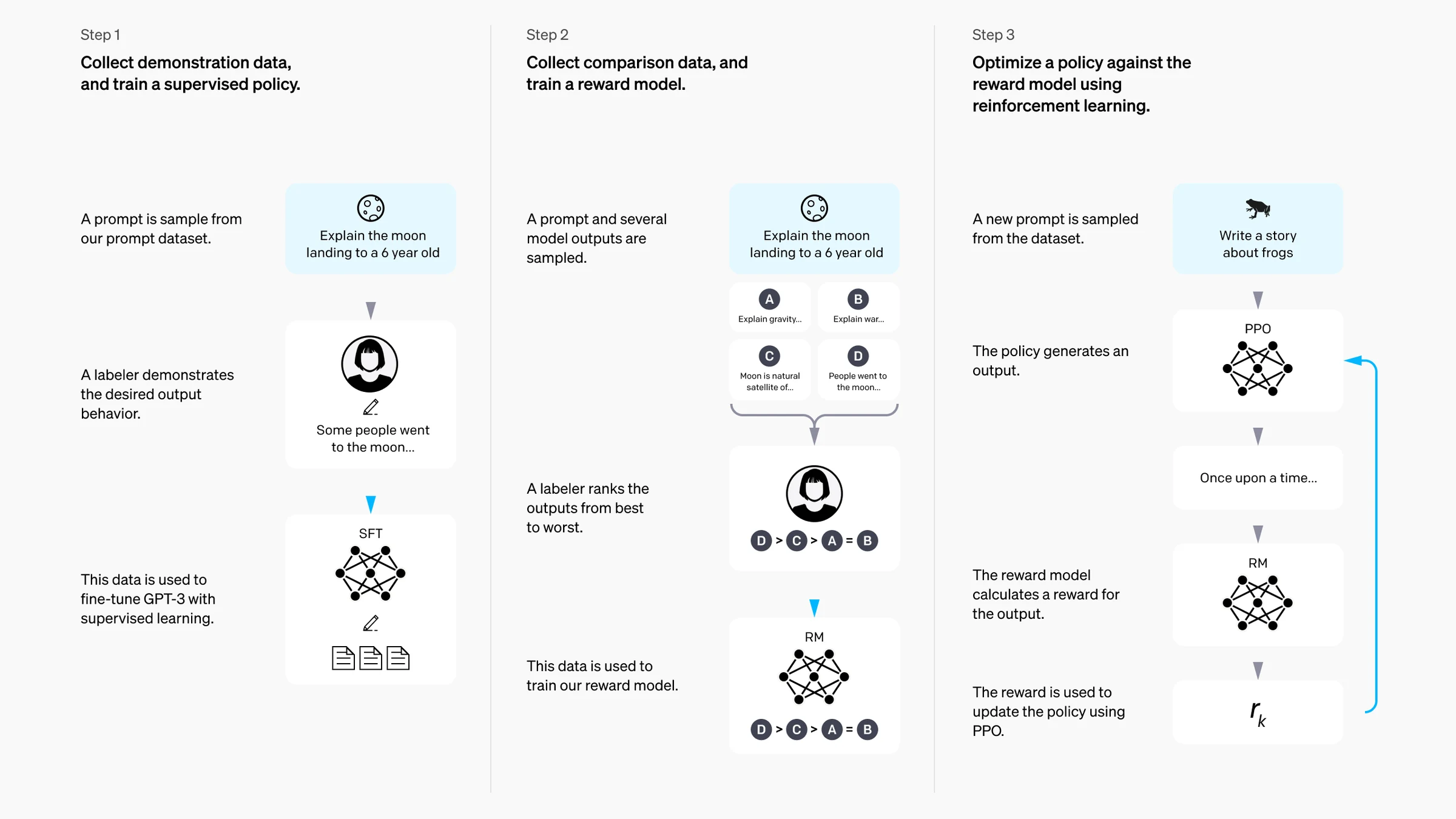
The scores given by the reward model represent a preference, not objective truth. If preference data coverage is insufficient or reward rule design is unreasonable, the model may simply learn to cater to the scoring method.
Actual models don't necessarily follow exactly the same pipeline. Some models use SFT plus DPO, some use SFT with a reward model and PPO, and others incorporate AI feedback, safety alignment, tool use training, and multi-turn dialogue data. The earlier pre-training, instruction fine-tuning, and post-training explained how model capabilities are formed. After model training is complete, the issues users more frequently encounter are how much content can be input at once, how much VRAM is needed at runtime, and what precision to choose for limited hardware.
After the model completes training, it enters the actual inference and deployment stage. Context length determines how many Tokens a single request can contain; the longer the context, the more material the model can read, but Attention computation and KV Cache usage also increase, affecting inference speed and VRAM requirements. The so-called context here refers to the system prompt, conversation history, current input, file content, tool descriptions, tool return results, and content already generated by the model in a single request, which can be expressed as: Context Usage = System Instructions + Conversation History + Current Input + Attachment Content + Tool Information + Model Output.
As mentioned earlier, a large model's context usage is not just the user's current input but is composed of multiple parts, including system instructions, prior conversation history, the user's current input, relevant content in attachments, information required for tool calls, and output already generated by the model. These all consume the model's context window, so as conversations grow longer, attachments increase, or tool information becomes more complex, the context space available for subsequent input and generation gradually decreases. For example, if a model indicates support for a context length of 128K, this usually represents the total order of magnitude of Tokens that can be processed in a single request. Whether output is included, what the maximum single output is, depends on the model and service interface limits. Typically, when context is exceeded, the platform may reject requests, truncate parts of the content, or automatically compress historical records.
To improve the model's inference efficiency and response quality in long document scenarios, content should be organized as much as possible before inputting materials, removing information irrelevant to the task, duplicate, or of low value, and clearly telling the model which sections, fields, or question areas to focus on, preventing the model from scattering attention across large amounts of irrelevant context. For particularly long materials that are difficult to process completely in one go, they can be segmented by chapter, topic, or fixed length first, letting the model complete information extraction, summarization, or analysis separately, then unifying and comprehensively evaluating the results from each part. For key conclusions, important data, or content that needs further verification, the model should also be required to indicate the corresponding original location, chapter, or page number, facilitating subsequent manual inspection and result tracing, thereby improving the overall processing accuracy, interpretability, and reliability.
Generative models based on the Transformer architecture typically generate Tokens one at a time. During generation, if the attention information for all previous Tokens were recalculated for each new Token, it would produce massive amounts of redundant work. Therefore, introducing a caching mechanism known as KV Cache is beneficial. KV Cache stores the Key and Value that have already been computed at each layer, so when generating the next Token, only the new parts need to be computed, improving generation speed. For each additional Token, every Transformer layer must save the corresponding K and V. Therefore, KV Cache grows with context length, output length, concurrency, and number of model layers.
For common Decoder-only models, the cache usage for a single sequence can be understood using the following simplified formula:
KV Cache Usage
\approx
2 \times Number of Layers
\times Number of Tokens
\times Number of KV Heads
\times Dimension per Head
\times Bytes per Number
After model weights are loaded, their usage is relatively fixed, but KV Cache changes with requests. Therefore, the same quantized model may run smoothly in short Q&A but still run out of VRAM when handling long documents or multiple concurrent users. For example, the same server might run normally when processing a single short meeting record, but if ten users simultaneously upload long records, the model needs to store KV Cache separately for multiple sequences, and VRAM pressure increases significantly. This also explains why, even if the model file fits in VRAM, computational resource consumption changes as text length and concurrency increase. Therefore, in practical deployment, KV Cache pressure can be reduced and computing service efficiency improved by shortening irrelevant context, limiting maximum generation length, reducing concurrency, using paged cache, or choosing models that use GQA or MQA structures.
Model files essentially store the current model structure and its related parameters, which are fundamentally a set of numbers. Drawing on principles from computer architecture, these parameters are typically expressed as combinations of 0s and 1s. Using different bit widths to represent the same value defines both the numerical range and precision. During model training, floating-point formats such as FP32, FP16, or BF16 are typically used for computation, representing a number with 32 bits or 16 bits of 0s and 1s. While more bits increase both numerical range and precision, actual resource consumption is also substantial. Therefore, quantization methods were proposed to further reduce resource consumption. Quantization converts these multi-bit floating-point values into lower-precision representations such as 8-bit INT8 or 4-bit INT4, reducing model file size and runtime resource usage. The following table shows the characteristics corresponding to different floating-point precisions:
Precision | Theoretical Bytes per Parameter | Typical Characteristics |
FP32 | 4 | Higher precision, larger resource usage |
FP16 / BF16 | 2 | Common training and high-precision inference format |
INT8 | 1 | Weights theoretically use about half of 16-bit |
INT4 | 0.5 | Weights theoretically use about one-quarter of 16-bit |
Actual quantization doesn't simply round all decimals; it maps a group of floating-point values to a finite range while storing scaling factors, zero points, or group information. Common approaches include compressing only model weights, quantizing both weights and activations, and post-training quantization after model training is complete. We need not worry excessively about numerical changes caused by quantization, because during generation, the model predicts the probability of each candidate Token as the next word, and during selection, it primarily concerns ranking and normalized scores. Therefore, while quantization does lose some precision, under strict controls, it can effectively balance the model's generation quality.
When selecting models, it's often necessary to determine whether VRAM is sufficient. The 7B, 14B, and 70B in model names typically represent approximately 7 billion, 14 billion, and 70 billion parameters respectively. Parameters are the numerical values learned during model training, distributed across modules such as Attention, feed-forward networks, and Embedding.
Parameter count cannot be directly equated with model file size; the precision used for each parameter must also be considered. When calculating only model weights, the following formula can be used:
Weight Usage ≈ Parameter Count × Bytes per Parameter
Parameter Scale | FP16 / BF16 | INT8 | INT4 |
7B | ~14GB | ~7GB | ~3.5GB |
14B | ~28GB | ~14GB | ~7GB |
32B | ~64GB | ~32GB | ~16GB |
70B | ~140GB | ~70GB | ~35GB |
The numbers in the table only represent the theoretical lower limit of model weights. Quantized models also need to store scaling factors and other information, and actual inference also requires KV Cache, intermediate computation results, inference framework workspaces, and concurrent request caches.
For example, a 14B model's INT4 weights are theoretically about 7GB, but on an 8GB graphics card there is almost no room left for KV Cache and runtime buffers. It might run with short context and single requests, but is prone to VRAM insufficiency when processing long documents. Using 12GB or 16GB VRAM is more comfortable. 70B INT4 weights are about 35GB, generally requiring more than 48GB VRAM. During deployment, options include using graphics cards with larger VRAM, multi-card setups, or using CPU memory for mixed inference.
General large models need to cover extensive knowledge and tasks. In specialized scenarios such as healthcare, finance, law, and code, they may not be familiar with industry terminology, business processes, and risk boundaries. Domain models are typically trained or adapted on a general base model using professional data and tasks, making the model more suitable for a particular domain. They don't necessarily need to be trained from scratch, nor are they simply made into domain experts through prompts alone. Common training and adaptation methods include:
It is important to distinguish between domain models and domain applications. Domain models have been trained with professional data, and professional capabilities are already embedded in model parameters. Domain applications can directly use general models, then connect to professional knowledge bases, rules, and tools. Practical systems often combine both approaches.
The legal Q&A system shown in the figure below first extracts keywords, then retrieves reference provisions from the legal vector database, and finally, the legal large model generates responses by combining evidence. This demonstrates that professional capability doesn't necessarily rely solely on model parameters; external materials are also an important component of domain applications.
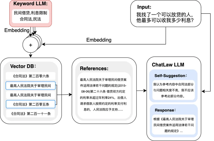
Professional data does not equal professional reliability. Medical models still need to check medical evidence and safety boundaries, legal models need to check legal provisions and citations, financial models need to check data timeliness and computational results, and code models need to be verified through running and testing. High-risk tasks in healthcare, law, and finance should also retain professional review and approval.
When using a model to organize meeting records, if the original text doesn't specify a responsible person but the model invents a name; when using a model to extract information from contracts, if the original text doesn't contain an amount but the model generates a specific number—these are all examples of model hallucination. Model hallucination refers to when a large model generates content that is linguistically fluent and structurally complete but inconsistent with facts, input materials, or verifiable sources. It may also manifest as fabricating non-existent policies, papers, or URLs, misidentifying people and times, or presenting unconfirmed discussions as established conclusions.
The core task of large models is to predict the next Token based on context; during generation, the model cannot verify whether each sentence is true. There are many causes of model hallucination. For example, pre-training data may contain errors or outdated information; user questions may lack key conditions; and evidence in long texts may be overlooked or truncated. If post-training designs reward functions that favor complete and fluent responses, it may also cause the model to continue generating even without sufficient basis.
Hallucinations produced by models are also diverse and can typically be classified as factual hallucination, attribution hallucination, reasoning hallucination, etc. Detailed classifications and typical manifestations are shown in the following table:
Type | Typical Manifestation |
Factual Hallucination | Names, dates, numbers, and events inconsistent with reality |
Attribution Hallucination | Fabricated papers, legal provisions, links, or sources |
Input Hallucination | Generating conclusions and fields not present in the original material |
Reasoning Hallucination | Errors in intermediate reasoning, but the response is expressed with certainty |
Tool Hallucination | Claiming to have read a file or called an interface when it actually didn't succeed |
In addition to general models, domain models trained with professional data can also produce hallucinations. Typically, professional data can improve domain performance but cannot guarantee that every answer is accurate. Knowledge base retrieval also cannot completely solve all hallucination problems. If retrieved materials are irrelevant, outdated, or themselves contain errors, the model may still arrive at incorrect conclusions, further leading to hallucinations.
Model hallucination is a relatively common problem in current applications. Simply adding a sentence like "don't fabricate" or "please ensure accuracy" to the prompt usually cannot fundamentally eliminate this risk. The model is fundamentally still predicting the most likely content based on context, and when input information is insufficient, materials contain conflicts, or the question itself exceeds the model's reliable knowledge range, it may still generate answers that appear plausible but are actually inaccurate. Therefore, reducing hallucination risk relies more on a complete set of input constraints, external verification, and human review mechanisms.
First, models should be provided with clear, relevant, and internally consistent materials as much as possible, reducing interference from irrelevant and conflicting information in the judgment process. For key content such as facts, numbers, policy provisions, and experimental results, the model can be required to simultaneously indicate corresponding sources, sections, page numbers, or original locations, making responses traceable for subsequent verification. For frequently updated knowledge such as news, policies, prices, regulations, and product parameters, one should not rely solely on the model's internal memory but should obtain the latest information through search engines, knowledge bases, databases, APIs, or other external tools, then have the model analyze based on these reliable materials.
Second, when the original material genuinely lacks certain information, the model should be explicitly required to mark it using phrases like "to be confirmed," "not provided in the original," or "cannot be determined based on existing materials," rather than completing it based on experience. For content suitable for structured verification—such as dates, amounts, ID numbers, statistical data, formulas, and code execution results—programs can be introduced for automatic verification, for example checking numerical ranges, field formats, computational results, and whether code can actually run, thereby avoiding the model generating results based solely on language generation.
Additionally, for important conclusions—especially those that affect business decisions, project acceptance, or user rights—a human review step should be retained. Fluent language expression and seemingly complete logic do not necessarily mean facts are correct, so "sounds like it's true" should not be directly equated with "is actually true." In high-risk scenarios such as healthcare, law, finance, and safety production, it should be made clear that the model is merely an auxiliary tool, and final conclusions need to be reviewed and confirmed by qualified professionals with appropriate experience.
Therefore, the core approach to reducing hallucination is not requiring the model to "always answer" but teaching the model to rationally stop when lacking reliable basis. When existing information is insufficient to support a conclusion, the most appropriate behavior may be to clearly state "which key materials are currently missing" and "which conclusions cannot be confirmed at this time," and further inform the user what data, documents, or evidence need to be supplemented. Compared to continuing to generate an answer that appears complete but lacks basis, this approach is generally more reliable and more suitable for practical business applications.