Artificial Intelligence Generated Content (AIGC) has been an important development direction in the field of artificial intelligence in recent years. Unlike traditional classification, prediction, and retrieval tasks, generative models aim to learn the probability distribution of data and generate new content under the guidance of conditions such as text and images.
From early Generative Adversarial Networks (GANs) and Variational Autoencoders (VAEs), to the widely adopted Diffusion Models and Diffusion Transformers (DiT) in recent years, generative models have continuously improved in generation quality, training stability, semantic understanding capability, and inference efficiency. Building on this foundation, text-to-image models such as Stable Diffusion, FLUX, Qwen-Image, and Z-Image have further advanced AIGC applications in content creation, advertising design, and marketing material production.
The core objective of generative models is to learn the underlying probability distribution and inherent patterns in training data, and to generate new samples conforming to that distribution under given conditions. Unlike classification and retrieval tasks, generative models do not select an answer from pre-given candidate results; instead, they use learned data patterns to generate new text, images, speech, or video content.
From a probabilistic modeling perspective, conditional generation tasks can be represented as: $p(x \mid c)$ represents the conditional probability distribution of the model generating content x given condition c. For example, the user's input Prompt, context, reference image, or other control information; x represents the target content to be generated. The process of model training is essentially learning the probability of various possible outcomes under different conditions; the process of model inference then produces concrete results based on this probability distribution.
Although large language models, image generation models, and video generation models all belong to generative models, the specific ways they achieve generation are not entirely the same.
Taking large language models as an example, current mainstream models typically use autoregressive generation to produce text. Given existing context, the model predicts the probability distribution of the next Token, selects or samples the next Token based on this probability distribution, adds the newly generated Token to the context, and continues predicting subsequent Tokens. By repeatedly repeating this process, complete text content is eventually formed.
Image generation models use different generation mechanisms. Taking diffusion models as an example, the generation process typically starts from random noise and gradually denoises under the guidance of conditions such as text prompts, allowing random noise to gradually form images with clear structure and semantics. Whether using autoregressive, diffusion, or other generation mechanisms, their common goal is to learn the distribution patterns of real data and generate new content conforming to these patterns based on given conditions.
సైన్ ఇన్ చర్చలో చేరండి
Generative models can generate new content, an important reason being that the model does not learn a specific text or image itself, but the statistical relationships and feature patterns that exist among a large amount of training data.
For example, after learning from a large number of beverage advertisement images, the model may gradually establish associations among visual concepts such as beverage bottles, ice cubes, water splashes, fruits, background colors, lighting, and commercial photography styles. When inputting "summer lime beverage commercial advertisement," the model can reorganize different visual elements based on these learned patterns to form new image results. The "generation" of generative models is not equivalent to finding an existing data entry from the training set; it is modeling and combining different features and concepts based on learned data distributions.
Another important characteristic of generative models is that generation results are diverse. For example, for the same prompt "a cat sitting by the window," the model may generate cats of different breeds, postures, and fur colors, and may also adopt different lighting, backgrounds, and image compositions. These results are semantically consistent with the input conditions, but the specific content is not entirely identical. The reason for this phenomenon is that the Prompt typically only imposes certain conditional constraints on the generated content rather than completely specifying the final result. Under given conditions, there are usually multiple reasonable results in the probability distribution learned by the model. In the actual generation process, factors such as sampling strategies and random seeds will further influence the final output. Unlike traditional tasks with deterministic answers, generation tasks typically do not have a unique optimal output; the same input conditions can correspond to multiple reasonable generation results.
Text generation technology plays a fundamental role in the development of modern generative AI. On one hand, large language models have driven the rapid popularization of AIGC technology; on the other hand, concepts such as Tokenizer, Embedding, Transformer, probability distribution, and sampling not only apply to text generation but will also repeatedly appear in subsequent text-to-image, multimodal generation, and other tasks. Especially in current AIGC systems, text Prompts have become an important way for users to control generated content. Whether generating a piece of text, an image, or a video, models typically need to first understand the natural language input by the user.
Natural language itself cannot directly participate in neural network computation. Before text is input to the model, it first needs to be segmented by a Tokenizer and converted to corresponding Token IDs. Tokens are the basic units for language models to process text; they can be a Chinese character, a complete word, or part of a word. The specific segmentation method is determined by the tokenization algorithm and vocabulary adopted by the model. Token IDs are essentially just the index numbers of Tokens in the vocabulary; their numerical values do not represent semantic relationships between Tokens. For example, two Tokens with close indices are not necessarily semantically similar. Therefore, before entering the neural network for computation, the discrete Token IDs need to be mapped to continuous high-dimensional vectors through an Embedding layer. This idea of using continuous vectors to represent language is an important foundation of modern natural language processing. In 2013, Mikolov et al. proposed Word2Vec, which learns distributed vector representations of words from large-scale corpora through neural networks. The basic idea originates from the distribution hypothesis in natural language, namely that words appearing in similar contexts usually have similar semantic or grammatical features.
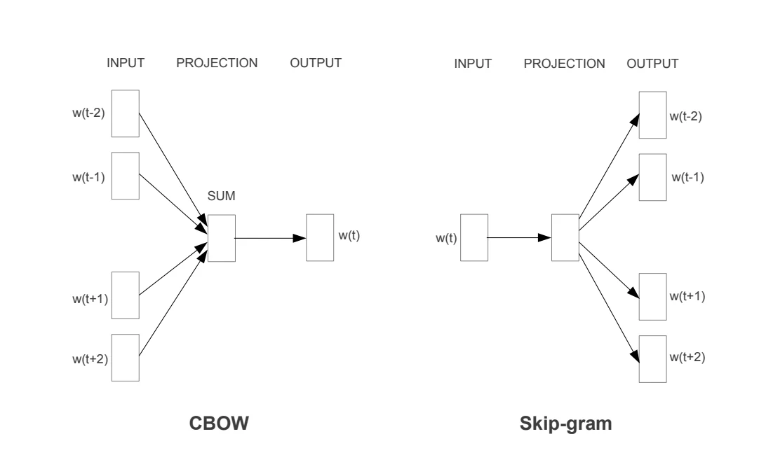
Word2Vec mainly includes two training structures: CBOW (Continuous Bag-of-Words) and Skip-gram. Both learn word vectors through the relationship between center words and context words, but their prediction directions are different.
CBOW predicts the center word based on context words. For a sequence composed of words, a center word is first selected, and words within a certain window range around it are used as context. The model uses the vector representations of these context words to predict the center word. For example, with "eat" as the center word, selecting "like" and "fresh" from its surroundings as context.
Skip-gram, on the other hand, predicts context words based on the center word. Compared to CBOW, its prediction direction is opposite. For the same word sequence, when "eat" is the center word, Skip-gram's training objective is to predict other words that may appear within a certain window range based on the vector representation of "eat," such as "like," "fresh," etc. The main difference between CBOW and Skip-gram is their training objectives: CBOW uses multiple context words to predict one center word; Skip-gram uses one center word to predict multiple context words. Despite their different prediction directions, their ultimate goal is to learn word vectors through a large amount of co-occurrence relationships between words. After training is complete, each word can be represented as a continuous vector of fixed dimensions.
The proposal of Word2Vec promoted the development of distributed word representations, but its representation method still has certain limitations. Word2Vec learns typical static word embeddings, where a word usually corresponds to a fixed vector after training and does not change with specific context. Modern language models further adopt contextual representations. Tokens first obtain initial vectors through the Embedding layer, then pass through multiple layers of neural networks, continuously updating their representations based on information from other Tokens in the sequence. Therefore, the same Token can form different hidden states in different contexts, thereby expressing semantics related to the current context. The significance of Word2Vec lies not only in proposing a specific word vector training method but also in promoting the widespread application of distributed representations in natural language processing. Language is no longer represented only through discrete symbols or indices but is also mapped to continuous vector spaces, enabling neural networks to further learn semantic and grammatical relationships between words. Subsequent natural language processing technology further focuses on how to use context to dynamically adjust word representations.
In 2017, the Transformer architecture was proposed. Transformer models relationships between different positions in a sequence through attention mechanisms and gradually became the core infrastructure of large language models. One of the most important mechanisms in Transformer is Self-Attention, as shown in the following figure:
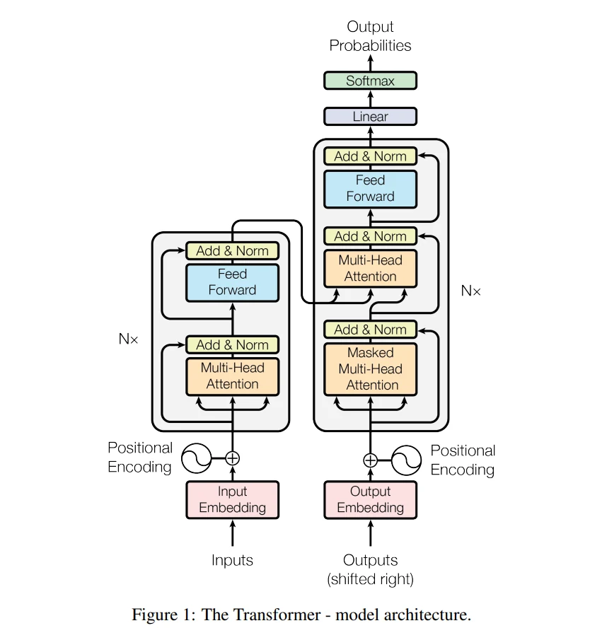
The main function of the self-attention mechanism is to allow the model, when processing a Token, to simultaneously consider information contained in other Tokens in the sequence and dynamically assign different attention weights based on the degree of association between them. Specifically, each Token's representation is mapped to Query (Q), Key (K), and Value (V). The model calculates attention weights through the matching degree between Query and different Keys, then uses these weights to perform weighted combination of the corresponding Values, thereby obtaining a new representation that incorporates contextual information.
Transformer is typically composed of multiple stacked network layers. In different layers, the model continuously updates each Token's representation, progressively incorporating richer contextual information. After processing through multiple layers of Transformer, the same Token can form different contextual representations in different contexts, thereby supporting the model's modeling of word meanings, syntactic structures, and more complex semantic relationships. The significance of Transformer lies not only in introducing a new network architecture but also in providing a mechanism that can effectively model contextual relationships. Modern large language models continuously improve language understanding and generation capabilities by expanding model scale, training data scale, and context length, all built upon the foundation of Transformer.
After Transformer performs contextual modeling on the input sequence, the language model has obtained Token representations incorporating contextual information. Building on this, generative language models need to further predict subsequent content. Mainstream generative large language models such as GPT typically use autoregressive generation, which progressively predicts and generates subsequent Tokens based on currently input or generated Tokens.
For a sequence composed of multiple Tokens, its generation probability can be decomposed into a series of conditional probabilities:
p(x_1, x_2, \ldots, x_T) = \prod_{t=1}^{T} p(x_t \mid x_1, x_2, \ldots, x_{t-1})
Where, $x_t$ represents the $t$-th Token to be generated currently, $x_1,x_2,\ldots,x_{t-1}$ represents previously input or generated Tokens. This formula indicates that the generation process of a complete text sequence can be decomposed into multiple consecutive next-Token prediction processes.
After the model calculates the probability distribution of the next Token, it needs to determine the actually output Token through decoding strategies. Different decoding strategies directly affect the stability, diversity, and creativity of text generation.
The most direct method is greedy decoding, which selects the Token with the highest probability at each step. This method has strong determinism, but consecutively selecting locally highest-probability Tokens does not necessarily yield text with optimal overall quality, and the generated content tends to be monotonous. To improve the diversity of generation results, generative language models can also use random sampling, selecting the next Token according to the probability distribution predicted by the model. Tokens with higher probabilities are more likely to be selected, but other reasonable candidate Tokens also have a chance of being selected. In practice, methods such as Temperature, Top-k, and Top-p are typically combined to further adjust the sampling process.
Temperature is used to adjust the smoothness of the probability distribution and can be represented as:
p_i =
\frac{\exp(z_i / T)}
{\sum_j \exp(z_j / T)}
Where, $z_i$ represents the Logit of the $i$-th Token, $T$ represents Temperature.
When $T$ is small, the advantage of high-probability Tokens is further enhanced, the model tends to select results with higher probabilities, and the generated content is typically more stable; when $T$ is large, the probability distribution is relatively flatter, low-probability Tokens get more opportunities to be selected, and the generation results typically have higher diversity.
Top-k retains only the $k$ candidate Tokens with the highest probability at each generation step, and resamples after renormalizing probabilities among these candidate Tokens. This method can filter out a large number of low-probability Tokens, reducing the possibility of clearly unreasonable content being selected.
Top-p does not fix the number of candidate Tokens; instead, it ranks probabilities from high to low and selects the smallest candidate set whose cumulative probability reaches threshold $p, then samples from this set. Therefore, Top-p can dynamically adjust the range of candidate Tokens based on the current probability distribution.
For example, when the model's prediction of the next Token is relatively certain, the cumulative probability of a small number of Tokens can reach the set threshold; whereas when the model has multiple reasonable candidate results, more Tokens are retained for sampling. Text generation actually includes two closely related processes: first, the language model calculates the probability distribution of the next Token based on context, then the decoding and sampling strategies determine the actually generated Token based on this probability distribution.
The model is responsible for learning which Tokens are more likely to appear in the current context, while the decoding strategy is responsible for deciding how to select specific results from these candidate Tokens. Together, they determine the accuracy, stability, and diversity of the final text.
In the development of deep learning generative models, Generative Adversarial Networks (GANs) represent a class of representative techniques. In 2014, Goodfellow et al. proposed GAN, which learns the distribution patterns of real data through adversarial training between two neural networks. Unlike traditional supervised learning, GAN does not directly specify what kind of images the generator should output; it also introduces a discriminator to evaluate the generation results and uses the discrimination results to continuously improve the generator. After its proposal, GAN was quickly applied to tasks such as image generation, face generation, image style transfer, super-resolution, and image editing, forming a series of representative models including CycleGAN, StyleGAN, and ESRGAN.
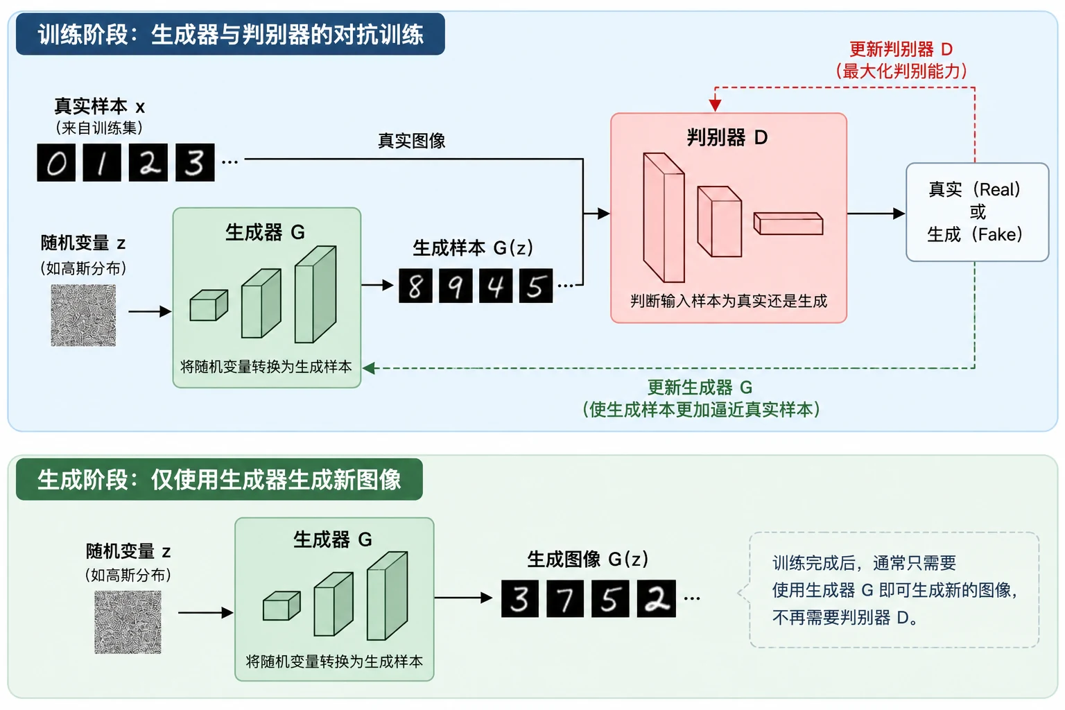
GAN learns the distribution of real data through adversarial training between two neural networks: the Generator and the Discriminator. As shown in the figure, during training, the Discriminator simultaneously receives real samples from the training set and generated samples from the Generator, and distinguishes between the two types of samples; the Generator continuously adjusts its own parameters based on feedback from the Discriminator, improving the similarity between generated samples and real samples.
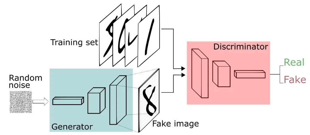
The Generator is denoted as G. Its input is typically a random variable z sampled from a simple probability distribution, such as a Gaussian or uniform distribution. After the Generator's nonlinear mapping, the random variable is transformed into a generated sample:
\hat{x}=G(z), \qquad z\sim p_z(z)
In image generation tasks, the Generator's objective is to progressively map low-dimensional or high-dimensional random representations into images with specific visual structures.
The Discriminator is denoted as D. Its input includes real samples x from the training set and generated samples G(z) from the Generator. By learning the feature differences between the two types of data, the Discriminator outputs the probability that the input sample comes from the real data distribution:
D(x)\in[0,1]
For real samples, the Discriminator hopes the output is close to 1; for generated samples, the Discriminator hopes the output is close to 0. The Generator and Discriminator have opposite optimization objectives. The Discriminator needs to continuously improve its ability to distinguish real samples from generated samples, while the Generator needs to continuously improve the authenticity of generated samples, making them more similar to real samples in terms of data features. The two networks form an adversarial relationship during the alternating optimization process. The original paper defines GAN's training objective as a minimax game:
\min_G \max_D V(D,G)
=
\mathbb{E}_{x\sim p_{\mathrm{data}}(x)}
[\log D(x)]
+
\mathbb{E}_{z\sim p_z(z)}
[\log(1-D(G(z)]
Where, $p_{\mathrm{data}}$ represents the real data distribution, $p_z$ represents the prior distribution of the random variable. The Discriminator $D$ improves its ability to distinguish real samples from generated samples by maximizing the objective function; the Generator $G$ gradually approaches the real data distribution by optimizing its own parameters.
GAN training typically adopts an alternating optimization approach. First, real samples and generated samples are used to update the Discriminator $D$, enabling it to learn the differences between the two types of data; then, gradient information from the Discriminator is used to update the Generator $G$, allowing the Generator to progressively improve generation results. As training continues, the capabilities of both the Generator and Discriminator change simultaneously, forming a dynamic adversarial learning process.
The Generator and Discriminator serve different functions in GAN. The Discriminator is primarily used in the training phase, providing optimization signals for the Generator through true/false classification; after model training is complete, if the task is only to generate new images, only the Generator is needed for inference:
GAN has received widespread attention in the field of image generation, an important reason being that its generation process is relatively direct. After model training is complete, it only needs to input random variables into the Generator, and a generation result can be obtained through a single forward computation. Compared to models that require multi-step iterative generation, GAN typically has higher generation efficiency, so it has been widely applied in tasks such as image generation, super-resolution, video enhancement, and interactive image processing. GAN's advantages are mainly manifested in the generation phase, while its training process is relatively complex, with the following main issues.
GAN requires simultaneously training the Generator and the Discriminator, and the two networks have mutually adversarial optimization objectives. When Generator parameters change, the generated data facing the Discriminator also changes; when Discriminator parameters change, the optimization signal received by the Generator also changes. Therefore, unlike ordinary supervised learning which optimizes under a relatively fixed objective function, GAN training is actually a constantly changing dynamic game process. If the Discriminator is too strong, generated samples may be easily identified and the Generator cannot obtain effective optimization signals; if the Discriminator is too weak, it cannot accurately reflect the differences between real samples and generated samples, and similarly cannot provide effective training feedback for the Generator. Therefore, maintaining a relatively stable training state between the Generator and Discriminator is an important issue in GAN model training.
Mode collapse is another typical problem in GAN training. Ideally, the Generator not only needs to generate samples with high visual quality but should also be able to cover different types and features in the real data. For example, assuming the training data contains faces of different ages, expressions, and appearance features, the Generator should be able to produce face images with corresponding diversity. However, in actual training, the Generator may tend to generate a small number of sample categories that are easier to receive higher evaluations from the Discriminator, and continuously produce similar results. At this point, individual generated images may have high visual quality, but the differences among a large number of generated results are small, unable to fully cover the diversity of real data. Mode collapse reflects an important problem in generative models: high single-sample generation quality does not mean the model has completely learned the real data distribution.
Regarding issues such as training instability, mode collapse, and generation quality, researchers have improved GAN from multiple aspects including network structure, loss functions, and training strategies, forming a large number of derivative models. These studies not only improved GAN's generation capabilities but also gradually expanded it from basic image generation to different tasks such as image translation, controllable image editing, and image super-resolution. Below, through several representative models, we introduce GAN's typical applications in these directions.
With the development of GAN technology, its application scope has gradually expanded from random image generation to tasks such as image translation, image editing, and image enhancement. Different models typically redesign generators, discriminators, loss functions, or training methods for specific tasks, forming GAN derivative models with different functions. Among them, CycleGAN, DragGAN, ESRGAN, and Real-ESRGAN respectively represent GAN's typical applications in unpaired image translation, interactive image editing, and image super-resolution.
In 2017, Zhu et al. proposed CycleGAN, primarily used to solve unpaired image-to-image translation problems. Unlike image translation methods that require paired training samples, CycleGAN does not require a one-to-one correspondence between source and target images; it only needs to provide data from two image domains separately to learn the translation relationship between them. For example, in the horse → zebra translation task, traditional methods typically need to prepare corresponding horse and zebra images, while CycleGAN only needs to separately prepare a set of horse images and a set of zebra images without establishing correspondence between the two sets of images. As shown below, CycleGAN consists of two generators and two discriminators, simultaneously learning image translation in both directions. Assuming horse images belong to image domain $X$, zebra images belong to image domain $Y$, Generator $G$ is responsible for completing the translation from $X$ to $Y$, and Generator $F$ is responsible for completing the translation from $Y$ to $X$:
G:X\rightarrow Y,\qquad F:Y\rightarrow X
Where, Discriminator $D_Y$ is used to judge whether the generated zebra images conform to the distribution of real zebra images, and Discriminator $D_X$ is used to judge whether the generated horse images conform to the distribution of real horse images. Therefore, CycleGAN actually contains two directional adversarial learning processes:
G + D_Y:Horse → Zebra
F + D_X:Zebra → Horse
Adversarial training in two directions alone cannot guarantee that translated images maintain correspondence with the original input. For example, when translating a horse image to a zebra, although the generated result may have realistic zebra textures, the horse's posture, position, or background structure may change significantly. That is, content consistency before and after translation cannot be fully guaranteed.
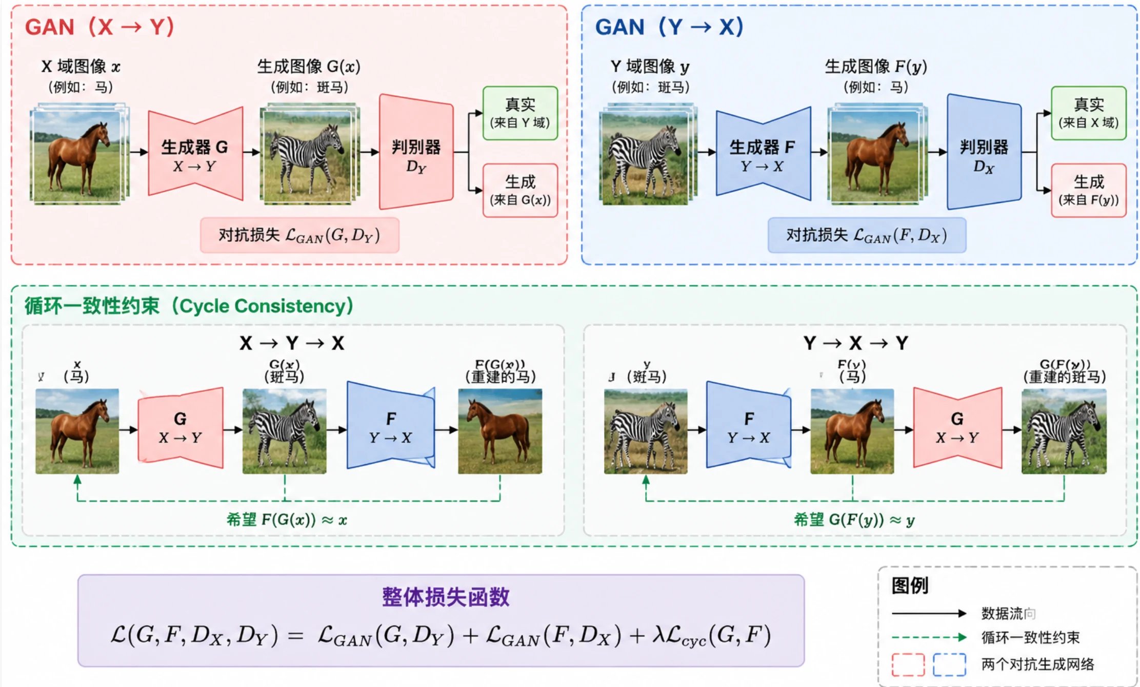
For this reason, CycleGAN further introduces cycle consistency constraints. As shown in the lower part of the figure, for horse image $x$ in image domain $X$, it is first translated to zebra image $G(x)$ through Generator $G$, then translated back to horse image through Generator $F$:
x\rightarrow G(x)\rightarrow F(G(x)
After one complete forward and reverse translation, the final result should be as close as possible to the original image:
F(G(x)\approx x
Similarly, for zebra image $y$ in image domain $Y$, it needs to satisfy:
G(F(y)\approx y
Therefore, the model forms two complete translation cycles: Horse → Zebra → Horse, Zebra → Horse → Zebra. CycleGAN introduces cycle consistency loss to constrain the two cycles:
\mathcal{L}_{\mathrm{cyc}}(G,F)
=
\mathbb{E}_{x\sim p_{\mathrm{data}}(x)}
\left[\|F(G(x)-x\|_1\right]
+
\mathbb{E}_{y\sim p_{\mathrm{data}}(y)}
\left[\|G(F(y)-y\|_1\right]
Where, the first term constrains the Horse → Zebra → Horse reconstruction result, and the second term constrains the Zebra → Horse → Zebra reconstruction result. The smaller the cycle consistency loss, the closer the image is to the original image in content and structure after bidirectional translation. CycleGAN's training mainly includes two parts: adversarial learning and cycle consistency constraints, which work together to enable CycleGAN to learn the mapping relationship between two image domains without paired training data, thereby achieving tasks such as horse-zebra translation and image style transfer.
In 2023, Pan et al. proposed DragGAN, which achieves interactive adjustment of object position, posture, and shape in generated images by setting control points and target points in the image. Unlike traditional pixel-level editing, DragGAN does not directly move pixels in the image; instead, it adjusts the latent representation of the GAN, causing the generated image to change according to the user-specified direction.
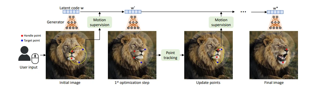
DragGAN's core process mainly includes motion supervision and point tracking. The user first selects the control point to be adjusted in the image and specifies the target position they wish to move to. For example, in the figure, by setting control points and target points near the lion's mouth, the lion's mouth gradually opens.
During the editing process, DragGAN keeps the pre-trained Generator's parameters unchanged and continuously optimizes the latent code $w$ input to the Generator. The initial image can be represented as:
I = G(w)
Where, $G$ represents the pre-trained GAN Generator, $w$ represents the latent code corresponding to the image. By adjusting $w$, the content and structure of the generated image $I$ can be changed. Motion supervision is used to push image features near the control point toward the target position. After one optimization, the latent code is updated from $w$ to $w'$, and the generated image changes accordingly. Since the original control point position may have shifted after the image changes, DragGAN also needs to re-determine the control point's position in the new image through point tracking, then continue with the next round of optimization, which is: set control point and target point → motion supervision → optimize latent code → generate new image → point tracking and update control point → continue optimization until approaching the target position. After multiple iterations, the control point gradually moves to the user-specified target position, ultimately yielding the edited image. Since this process is optimized in the generation space learned by GAN, the model not only changes the specified position but can also make corresponding adjustments to surrounding related structures.
DragGAN's key is not simply dragging pixels; it converts the user's drag operation into iterative optimization of the GAN's latent representation, and through motion supervision and point tracking, controls the semantic structure in the image to move toward the specified position. This method demonstrates GAN's application capability in controllable image editing, enabling users to intuitively adjust object posture, expression, and shape through point-based operations.
Image super-resolution is one of GAN's typical application directions, with the objective of generating images with higher resolution and richer visual details from low-resolution images. Unlike simple interpolation upscaling, super-resolution models need to reconstruct missing high-frequency textures and local structures based on existing image content. In 2018, Wang et al. proposed ESRGAN[ESRGAN], further improving the network structure, adversarial loss, and perceptual loss based on existing research to improve the texture performance and visual quality of super-resolution images.
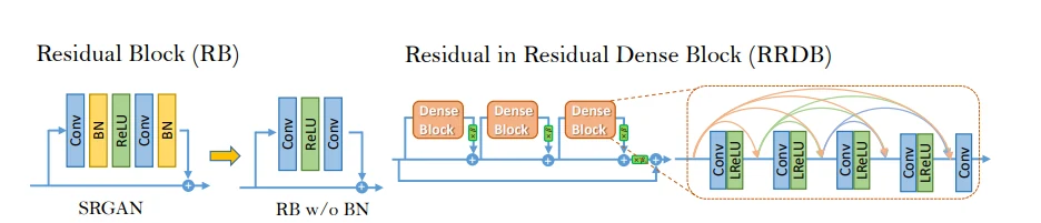
An important improvement in ESRGAN's network structure is the introduction of the Residual-in-Residual Dense Block (RRDB) structure. SRGAN's Generator mainly uses ordinary Residual Blocks (RB), which include convolutional layers, Batch Normalization (BN), and activation functions. ESRGAN first removes the BN layer from the residual blocks and further combines multiple dense connection modules into RRDB.
As can be seen from the figure, RRDB is internally composed of multiple Dense Blocks and combines dense connections with residual connections. Within Dense Blocks, different convolutional layers use dense connections, where subsequent layers can receive and utilize features extracted from multiple previous layers; between multiple Dense Blocks and outside RRDB, features are further transmitted through residual connections. This structure can strengthen information transmission and feature reuse between different layers, improving the network's modeling capability for image textures and detail features. In addition to network structure improvements, ESRGAN also optimizes the training objective. Traditional super-resolution methods, if primarily trained with pixel-level error, tend to generate relatively smooth results; although pixel error may be smaller, some edges and high-frequency textures tend to become blurred. ESRGAN further combines perceptual loss and adversarial training, allowing generation results to obtain clearer, more natural texture details while maintaining overall content.
Generative super-resolution is not equivalent to recovering lost original information. When some high-frequency information in low-resolution images has been lost, existing pixels alone usually cannot uniquely determine original details. ESRGAN actually combines the input image with image priors learned during training to generate visually reasonable textures. Although generated results may be clearer, some details may not be entirely consistent with the original high-resolution image. This characteristic makes ESRGAN more suitable for image enhancement tasks that emphasize visual quality. In scenarios with high requirements for information authenticity such as medical imaging, archival forensics, and scientific research images, generative super-resolution results should be used cautiously.
GAN learns real data distribution through adversarial training between Generator and Discriminator, while Variational Autoencoder (VAE) adopts a different generation approach: first encoding input data into a continuous latent space, then sampling from the latent space, and generating or reconstructing data through a decoder. In 2013, Kingma and Welling proposed the Auto-Encoding Variational Bayes (AEVB) method and provided the subsequently widely used VAE training framework. VAE combines neural networks with variational inference, enabling the model to learn latent representations with probabilistic structure through end-to-end training.
VAE's basic structure consists of an Encoder and a Decoder. The Encoder is responsible for compressing input data into a lower-dimensional latent space, while the Decoder recovers input data based on latent representations. Ordinary autoencoders typically encode input $x$ directly into a deterministic latent vector $z$, then use the decoder for reconstruction. The biggest difference between VAE and ordinary autoencoders is that the Encoder does not directly output a deterministic latent vector; instead, it outputs the parameters of the probability distribution of the latent variable.
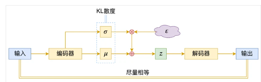
In the figure above, VAE's Encoder does not directly convert input data $x$ into a fixed latent vector; it also outputs two parameters: mean $\mu$ and standard deviation $\sigma$. These two parameters together determine the probability distribution of latent variable $z$. $\mu$ determines approximately where the latent variable is located, and $\sigma$ indicates how much variation range it can have around this position.
VAE models the latent variable as a Gaussian distribution:
q_{\phi}(z\mid x)
=
\mathcal{N}
\left(
z;\mu_{\phi}(x),
\operatorname{diag}\left(\sigma_{\phi}^{2}(x)\right)
\right)
Where, $q_{\phi}(z\mid x)$ represents the latent variable distribution obtained by the Encoder based on input $x$. Unlike ordinary autoencoders that directly obtain a deterministic $z$, VAE obtains a distribution that can be sampled, so the same input can yield different latent representations within a certain range. Next, the model needs to obtain a specific latent variable $z$ from this distribution and send it to the Decoder. To introduce randomness while ensuring the model can perform normal backpropagation, VAE uses the reparameterization trick. The model first samples a random variable $\epsilon$ from a standard normal distribution, then combines the $\mu$ and $\sigma$ obtained by the Encoder to compute latent variable $z$:
z=\mu+\sigma\odot\epsilon
It can be understood that $\mu$ determines the position, $\sigma$ determines the variation range, and $\epsilon$ provides randomness; together they produce the final latent variable $z$. This approach separates random sampling from the computation process of network parameters, allowing gradients to still propagate through $z$ to the Encoder, thereby enabling end-to-end training of the entire VAE. After obtaining latent variable $z$, the Decoder generates reconstruction result $\hat{x}$ based on $z$. VAE's entire process can be summarized as: input data → Encoder → latent distribution → sample to get $z$ → Decoder → reconstructed data.
VAE also needs to simultaneously consider two objectives during training: on one hand, it hopes the Decoder's generated results are as close as possible to the original input; on the other hand, it hopes the latent distributions corresponding to different inputs are not too disordered but form a relatively continuous and regular latent space. Therefore, VAE's training objective consists of both reconstruction and KL divergence terms, typically represented through the Evidence Lower Bound (ELBO):
\mathcal{L}_{\mathrm{ELBO}}
=
\mathbb{E}_{q_{\phi}(z\mid x)}
\left[
\log p_{\theta}(x\mid z)
\right]
-
D_{\mathrm{KL}}
\left(
q_{\phi}(z\mid x)
\parallel
p(z)
\right)
Where, the first term can be understood as how well the reconstruction is performed, measuring whether the Decoder can recover input data based on $z$; the second term can be understood as whether the latent space is sufficiently regular, constraining the latent distribution obtained by the Encoder through KL divergence to make it close to the pre-set prior distribution. These two objectives need to work together. If only reconstruction quality is considered, although the model can recover input well, the latent space may be quite scattered, making it inconvenient to sample directly from it; after adding KL divergence constraints, the latent representations of different samples are constrained by a unified prior distribution, making the latent space more regular and more suitable for sampling and generation.
From the generation process perspective, VAE already has complete generation capability. After training is complete, instead of inputting the original image, latent variable $z$ can be directly sampled from a standard normal distribution and input into the Decoder to generate new images. Theoretically, this process can work because during training, the latent distribution generated by the Encoder is continuously constrained through KL divergence to approach the pre-set standard normal distribution. However, in actual training, the latent distribution generated by the Encoder usually cannot completely match the standard normal distribution. If the constraint is too strong, although the latent space is more regular, some image information may be lost; if the constraint is too weak, the latent space distribution may not be regular enough, causing $z$ obtained by directly sampling from the standard normal distribution to fall in unfamiliar regions of the model, thereby affecting decoding results.
At the same time, VAE needs to balance between reconstruction quality and latent space regularity. Classic VAE's training objective emphasizes modeling the overall data distribution and latent space, tending to lose some high-frequency textures and local details during image generation, with generated results often being relatively smooth. This is also a clear distinction between VAE and GAN in image generation effectiveness. GAN directly constrains the authenticity of generated images through the Discriminator, typically producing sharper textures; VAE focuses more on the continuity and probabilistic structure of the latent space, with certain limitations in directly generating high-quality images.
With the development of generative models, VAE's role has gradually shifted from directly generating final images to serving as an encoding and decoding tool between image space and latent space. A representative application is the Latent Diffusion Model (LDM). Early diffusion models directly performed noise addition and denoising in pixel space. When image resolution is high, the model needs to repeatedly process a large number of pixels, resulting in high computational costs. The latent diffusion model proposed by Rombach et al. transfers the diffusion process to a compressed latent space, thereby reducing the data dimensions that the diffusion model needs to process. In this structure, the Encoder first compresses the original image into a latent representation: original image → Encoder → latent representation. These latent representations no longer directly save each pixel but retain the main structure and visual information of the image in a more compact form. Subsequently, the diffusion model performs noise addition and denoising in this latent space rather than directly processing the original high-resolution image. After the diffusion model completes generation, the Decoder restores the generated latent representation to pixel space: generated latent representation → Decoder → final image. VAE is responsible for compressing and restoring images, while the diffusion model is responsible for generating image content in the latent space. This approach fully utilizes VAE's latent representation capability. The diffusion model no longer processes high-dimensional original pixels but processes compressed image features, thereby significantly reducing the computational cost of subsequent diffusion and denoising processes.
VAE itself has certain limitations in directly generating high-quality images, but its Encoder, latent space, and Decoder structure have become important components of modern latent diffusion models. This also reflects the change in VAE's role: gradually evolving from an independent generative model to a latent representation module in high-quality image generation systems.
GAN typically uses the Generator to complete image generation through a single forward computation, and VAE can also start from latent variables and obtain generation results directly through the Decoder. For complex high-dimensional images, having the model complete the mapping from random variables to complete images in one step is not easy. Diffusion models adopt a different approach, splitting the complex image generation task into multiple relatively simple steps, with each step making only a small adjustment to the current result, gradually obtaining the complete image through multiple iterations. The model is not required to generate the final result in one step; instead, it gradually completes generation through multiple denoising steps.
Diffusion models mainly contain two processes in opposite directions: forward diffusion and reverse denoising. Forward diffusion starts from real data $x_0$ and continuously adds small amounts of random noise to it. As the time step $t$ increases, the original information in the image gradually decreases and noise gradually increases, eventually approaching random Gaussian noise. In the classic DDPM, noisy data at any time step can be directly constructed from the original data $x_0$:
x_t
=
\sqrt{\bar{\alpha}_t}x_0
+
\sqrt{1-\bar{\alpha}_t}\epsilon
Where:
\epsilon\sim\mathcal{N}(0,I)
,
x_0
represents the original data, $\epsilon$ represents random Gaussian noise, $\bar{\alpha}_t$ is used to control the proportion of original data and noise at the current time step. The later the time step, the less original information and the more noise. Different time steps correspond to different noise levels, and how these noise levels change is determined by the noise scheduling strategy.
Forward diffusion itself does not require model learning. During training, data with different noise levels can be directly constructed according to pre-defined rules. What the model truly needs to learn is the opposite process, that is, how to gradually recover clearer data from noisy data. During generation, the model starts from random noise, performing a certain degree of denoising at each step: random noise → preliminary structure → outline gradually becomes clear → texture gradually forms → final image. This mechanism splits a complex generation task that would be completed in one step into multiple relatively simple local correction tasks. The model does not need to predict the complete image at once; it needs to continuously adjust based on the current state, which is one of the important reasons why diffusion models can achieve high-quality generation.
In classic DDPM, two processes in opposite directions are established: the forward diffusion process continuously adds noise to real data, while the reverse generation process learns how to gradually remove noise, allowing random noise to eventually recover to images with real data characteristics.
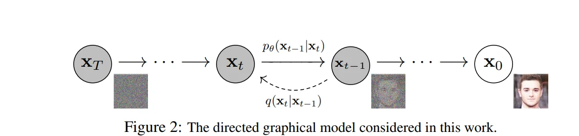
$x_0$ represents the real image. As forward diffusion continuously adds Gaussian noise, the data passes through $x_1,x_2,\ldots,x_T$ in sequence, and eventually $x_T$ approaches random Gaussian noise. The dashed line $q(x_t\mid x_{t-1})$ in the figure represents the forward diffusion process, while $p_\theta(x_{t-1}\mid x_t)$ represents the reverse generation process that the model needs to learn. The forward process can be understood as: real image x₀ → x₁ → x₂ → …… → xₜ → …… → random noise xT, while actual image generation proceeds in the opposite direction: random noise xT → …… → xₜ → xₜ₋₁ → …… → final image x₀. The key question of DDPM is how to let the model learn to obtain $x_{t-1}$ with less noise from current $x_t$.
In DDPM, the reverse process is parameterized by a neural network. An important and commonly used approach is to have the neural network predict the noise added to $x_t$. During training, starting from real image $x_0$, a random time step $t$ is selected and Gaussian noise
\epsilon\sim\mathcal{N}(0,I)
is sampled. According to the forward diffusion process, the noisy image corresponding to time step $t$ can be directly constructed:
x_t
=
\sqrt{\bar{\alpha}_t}x_0
+
\sqrt{1-\bar{\alpha}_t}\epsilon
Subsequently, the noisy image $x_t$ and time step $t$ are input to the neural network, and the model predicts the noise
\epsilon_\theta(x_t,t)
, where $\theta$ represents the parameters of the neural network. Since the real noise $\epsilon$ added during training is known, the difference between the model-predicted noise and the real noise can be directly compared. DDPM's training process can be understood as: first actively adding different levels of noise to real images, then training the model to identify what noise was added. After extensive training, the model can handle data at different time steps and different noise levels, and use noise prediction results to construct the reverse process $p_\theta(x_{t-1}\mid x_t)$ shown in the figure. During the generation phase, real images are no longer needed; instead, starting directly from Gaussian noise, the model first obtains $x_{T-1}$ with less noise from $x_T$, then obtains $x_{T-2}$ from $x_{T-1}$, and so on:
x_T
\rightarrow
x_{T-1}
\rightarrow
x_{T-2}
\rightarrow
\cdots
\rightarrow
x_1
\rightarrow
x_0
.
As the reverse process continues, the overall structure, outline, and texture of the image gradually emerge from the random noise, ultimately yielding the complete generated image. DDPM does not have the model predict the complete image from noise at once; instead, it learns denoising capabilities at multiple noise levels, then gradually completes generation through multiple reverse iterations. This approach reduces the difficulty of single-step generation tasks and avoids the adversarial training between Generator and Discriminator in GAN. However, multi-step sampling means that generating one image requires multiple neural network inference executions, so slow inference speed has also become one of the main limitations of classic DDPM.
DDPM describes image generation as a step-by-step denoising process, adding noise to real data during training and having the model learn to predict noise; during generation, starting from random noise, the image is gradually obtained through multiple reverse denoising steps. Flow Matching adopts a different descriptive approach. It constructs a continuous probability path between the random noise distribution and the real data distribution, and trains the model to learn the direction of change along this path, allowing random noise to gradually transform into real data along the learned direction.
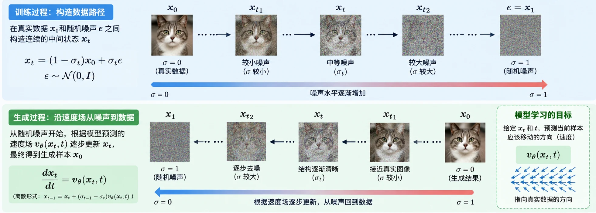
From the implementation perspective, Flow Matching mainly includes three stages: path construction, velocity field learning, and generation sampling.
During training, a sample $x_0$ is first sampled from the real data distribution, and random noise $\epsilon$ is sampled from a standard Gaussian distribution. To establish a connection between real data and random noise, a series of continuous intermediate states can be constructed between them. A relatively intuitive approach is to use linear interpolation:
x_t=(1-\sigma_t)x_0+\sigma_t\epsilon
, where $\sigma_t$ controls the proportion of real data and random noise in the current state. For ease of illustration, let:
\sigma_0=0,\qquad \sigma_1=1
, when $\sigma_t=0$:
x_t=x_0
This corresponds to real data; when $\sigma_t=1$:
x_t=\epsilon
This corresponds to random noise.
As $\sigma_t$ gradually increases from 0 to 1, $x_t$ can represent a series of continuous intermediate states between real data and random noise: real data → slight noise → moderate noise → heavy noise → random noise. During training, by randomly selecting different $t$, intermediate states at different positions can be obtained, providing training samples for the model to learn the change patterns along the entire path. Compared to the pre-defined step-by-step noise addition process in DDPM, Flow Matching is more concerned with how to define the continuous path connecting two distributions and how data should change along this path.
After constructing the continuous path, the next step is to determine the direction and speed of data changes on the path. Flow Matching uses a neural network to learn a velocity field
v_\theta(x_t,t)
, where $x_t$ represents the current intermediate state, $t$ represents the current time position, and $v_\theta(x_t,t)$ represents the model-predicted change velocity at the current position. For the linear path above:
x_t=(1-\sigma_t)x_0+\sigma_t\epsilon
During training, the target velocity can be obtained from the known real data $x_0$ and random noise $\epsilon$, and the neural network can be trained to predict the corresponding velocity based on the current state $x_t$ and time $t$. Flow Matching's training objective is to train the model to predict the data change velocity corresponding to a position, given the intermediate state $x_t$ and time $t$ on the path. After the model learns from a large number of training samples, velocities at different positions together form a velocity field. This velocity field describes how data should change at different positions in the data space, thereby providing direction for subsequent data generation from random noise.
The training phase establishes the path between real data and random noise and learns the velocity field on the path. The generation phase starts from random noise and uses the learned velocity field to gradually move toward the real data distribution. This process can be represented as: random noise → intermediate state → data structure gradually forms → final generated data,
x_{t-1}
=
x_t+
(\sigma_{t-1}-\sigma_t)
v_\theta(x_t,t)
The model re-predicts velocity at each time step based on the current state and updates $x_t$. After multiple iterations, the initial random noise gradually transforms into generated data with complete structure and semantic information.
From the modeling perspective, both DDPM and Flow Matching use simple random distributions as the generation starting point, but their descriptions of the generation process differ. DDPM mainly describes data changes through forward diffusion and reverse denoising, typically learning noise prediction; Flow Matching constructs a continuous path connecting noise and real data, learns the velocity field on the path, then starts from random noise and gradually generates data along the velocity field.
Text-to-Image refers to automatically generating corresponding images based on natural language descriptions. Compared to ordinary image generation, Text-to-Image not only requires the model to generate images with high visual quality but also needs to correctly understand the subject, attributes, quantity, position, style in the text, and the relationships between different objects. During the development of Text-to-Image, the technical focus has also gradually shifted from "whether images can be generated from text" to "whether complex instructions can be accurately understood and generation can be completed with higher quality, higher efficiency, and stronger controllability."
Early Text-to-Image research was mainly based on generative models such as GAN. The basic method was to first encode text into vectors, then use text features as conditional input to the Generator, making generation results consistent with text descriptions. This stage demonstrated the feasibility of Text-to-Image, but early GAN still had significant limitations in complex scene generation, text semantic understanding, and training stability. Especially when prompts contained multiple subjects, complex spatial relationships, or longer text descriptions, the model found it difficult to accurately restore all semantics. In 2021, OpenAI released DALL·E, using a Transformer-based autoregressive approach to process text and image Tokens, making Text-to-Image models achieve significant progress in complex concept combinations, attribute control, etc., and also driving the development of large-scale Text-to-Image models. At the same time, diffusion models began to enter the Text-to-Image field. GLIDE combined text conditions with diffusion models and studied CLIP Guidance and Classifier-Free Guidance, demonstrating that diffusion models could generate images with high visual quality under text control. In 2022, Google's Imagen further combined large language model text understanding capabilities with diffusion model image generation capabilities. Imagen used pre-trained T5 as the text encoder, converting Prompts to text semantic representations, then using them as conditional input to the diffusion model. Research showed that enhancing the text encoder's semantic understanding capability could further improve the consistency between generated images and text descriptions. With the development of models such as DALL·E, GLIDE, and Imagen, Text-to-Image gradually formed a relatively clear technical flow: text encoder → text semantic representation → diffusion generation model → step-by-step denoising → generated image; diffusion models, with their good generation quality and training stability, gradually became an important technical route in the Text-to-Image field.
Early diffusion models typically performed multiple noise additions and denoising directly in pixel space. As image resolution continuously increased, directly processing large numbers of pixels brought high training and inference costs. In 2022, Rombach et al. proposed the Latent Diffusion Model (LDM), transferring the diffusion process from pixel space to a compressed latent space (refer to LDM introduction in 14.4.3). The significance of Stable Diffusion lies not only in improving Text-to-Image quality but also in driving the development of an open-weight Text-to-Image ecosystem. Around its latent diffusion architecture, a large number of extension technologies have gradually formed, including LoRA, ControlNet, image-to-image, and local inpainting, making Text-to-Image gradually develop from a simple image generation tool into a complete visual content production system.
Early diffusion models typically used U-Net as the denoising network. U-Net, through multi-scale feature extraction and skip connections, could preserve the spatial structure of images relatively well, so it was long used as an important backbone network for diffusion models. With the continuous expansion of generative model scale, researchers began exploring using Transformers to replace U-Net to achieve better model scalability. In 2022, Peebles and Xie proposed the Diffusion Transformer (DiT), using Transformers to replace the commonly used U-Net backbone network in diffusion models. The model first divides the image representation in latent space into multiple Patches and converts them into Token sequences, then uses Transformers to model these Tokens. The DiT architecture is shown below:
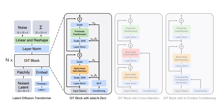
DiT research further showed that the model's computational scale could be expanded by increasing the depth, width, and input Token count of the Transformer. In the original paper's experiments, as model computational volume increased, generation quality generally showed a continuously improving trend, demonstrating that the Transformer architecture has good scalability in diffusion models. DiT's significance lies not only in replacing U-Net with Transformers, but more importantly in providing a new infrastructure for subsequent large-scale image generation models. Since then, Transformers have gradually become an important technical route for Text-to-Image models, and further developed into multimodal Transformer architectures that simultaneously process text Tokens and image Tokens, laying the foundation for next-generation Text-to-Image models such as Stable Diffusion 3 and FLUX.1.
With Transformers gradually becoming an important backbone network for Text-to-Image models, the image generation process itself is also continuously evolving. The previously introduced DDPM mainly describes data generation through "forward noise addition — learning reverse process — step-by-step denoising," while Flow Matching describes the transformation process from simple distributions to real data distributions from the perspective of continuous probability paths and velocity fields. In 2024, Stable Diffusion 3 related research further combined Rectified Flow with Transformers for high-resolution Text-to-Image. This work proposed a new Multimodal Diffusion Transformer (MMDiT) architecture.
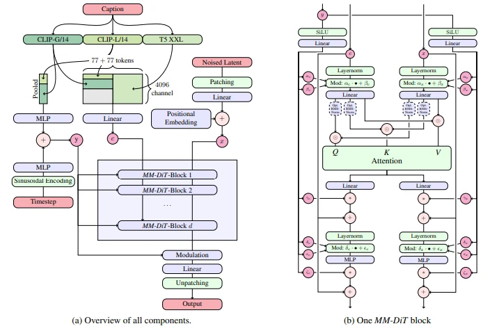
Unlike early DiT which mainly processed image latent Tokens, MMDiT processes text and image representations using independent parameters, while achieving information interaction between the two modalities through joint attention, thereby enhancing the model's understanding of text content, text rendering, and complex prompts. FLUX.1 released in the same year continued the technical route of combining Transformers with Flow Matching. FLUX.1 series models adopt a hybrid architecture composed of Multimodal Transformer Blocks and parallel Diffusion Transformer Blocks, and are trained based on Flow Matching. The publicly available FLUX.1 model scale reaches 12B parameters, further reflecting the trend of Transformer image generation models toward large-scale development. Starting from this stage, the technical focus of Text-to-Image models has no longer been limited to improving image visual quality but has gradually expanded to directions such as complex Prompt understanding, text-in-image generation, high-resolution generation, few-step sampling, and image editing. Text and image have also increasingly entered Transformers in Token form, achieving cross-modal information interaction through attention mechanisms. This change has also laid the foundation for more efficient and unified multimodal generation models.
With the continuous improvement of Text-to-Image model scale and generation quality, practical applications of models have begun to face new problems. On one hand, large-scale generation models typically require high computational resources and many sampling steps; on the other hand, practical AIGC applications are no longer limited to single Text-to-Image tasks but also need to simultaneously support image understanding, image generation, image editing, and reference image generation capabilities. Therefore, reducing generation costs and unifying multimodal capabilities have gradually become important development directions for Text-to-Image models.
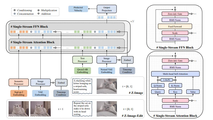
Z-Image series adopts the Scalable Single-Stream Diffusion Transformer (S3-DiT) architecture with a model scale of 6B parameters. An important feature of S3-DiT is its single-stream architecture, which concatenates text Tokens, visual semantic Tokens, and image VAE Tokens in the sequence dimension, then inputs them into a unified Transformer for processing. Compared to dual-stream structures that process different modalities separately, this approach can complete interactions between different types of information in a unified data flow. Z-Image-Turbo demonstrates an important development direction of modern Text-to-Image models: while maintaining strong generation capabilities, reducing inference costs through model distillation and few-step sampling, making large-scale Transformer image generation models more suitable for practical deployment.
SenseNova-U1.5-8B-MoT moving from Text-to-Image toward unified multimodal, in addition to improving generation efficiency, another important direction is unifying previously relatively independent multimodal understanding and multimodal generation capabilities. SenseNova-U1 released in 2026 proposed the NEO-unify architecture, attempting to simultaneously achieve multimodal understanding and generation in a unified model. Building on this, SenseNova-U1.5-8B-MoT further enhanced image generation and editing capabilities. According to official release information, the official version of SenseNova-U1.5-8B-MoT was released in August 2026, further improving instruction following, text and layout generation, native 4K image generation, image editing, and visual control capabilities.
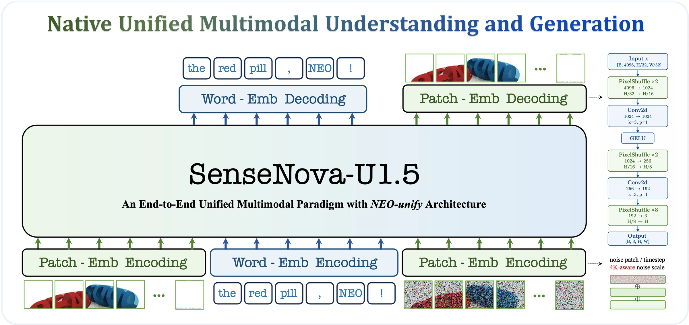
SenseNova-U1.5 is built on the NEO-unify unified multimodal architecture and adopts a new image Patch encoding and decoding mechanism. The model can not only generate images based on text descriptions but also combine input images with natural language instructions to complete image-to-image, image editing, and visual control tasks. This means Text-to-Image models are gradually evolving from simple content generation tools into unified multimodal models capable of simultaneously handling understanding and generation tasks.