After fine-tuning the model, it can answer questions as required. But when you put several responses together, some will be good and some will be bad, and some will look more comfortable to read.
Take a refund consultation for example. Both responses tell the user where to apply. One response only gives the operation entry, while the other also explains that review is needed and whether a refund is possible depends on the order situation. Both responses mention refunds, but the latter explains the situations the user might encounter next more clearly and reduces misunderstandings.
When we did SFT earlier, we organized such responses into examples for the model to learn from. Now we can also put different responses to the same question together, tell the model which one we prefer, and what the evaluation criteria are.
This is preference alignment. Let's start here.
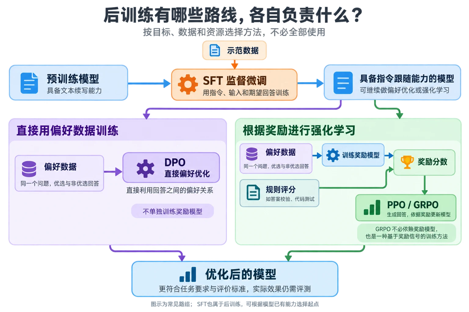
The main purpose of post-training for large models is to help base models that already have text continuation capability gradually become able to better conduct direct conversations, follow instructions, and complete specific tasks. Post-training is not a fixed algorithm but a general term for a group of training methods. Common methods include SFT, preference optimization, reward model training, and reinforcement learning. Different models choose different combinations based on training objectives, data conditions, and costs.
Among them, SFT mainly uses data in the form of "instructions, inputs, and expected responses" to let the model learn how to understand tasks, follow instructions, and answer in the expected format and manner. On this basis, preference data can be further used for alignment, such as constructing preferred and non-preferred responses for the same question, letting the model learn human or business evaluation criteria. Preference data can be used to train reward models, converting human preferences into computable reward scores, which are then combined with reinforcement learning methods like PPO and GRPO to continuously optimize the model's generation strategy. It can also directly use methods like DPO to write the preference relationship between preferred and non-preferred responses directly into the training objective without separately training a reward model.
Therefore, there is no fixed process for post-training large models. SFT, reward models, PPO, GRPO, and DPO also serve different responsibilities. SFT is mainly used to establish basic instruction-following capability, reward models are responsible for providing quantifiable evaluation signals, PPO and GRPO further optimize generation strategies based on reward signals, while DPO directly uses preference data to complete model alignment. In actual training, these methods are not all used, nor are they necessarily combined in exactly the same order, but are flexibly chosen based on model capabilities, task objectives, and training resources.
Sign in to join the discussion
SFT (Supervised Fine-Tuning) uses organized input and expected output to continue training the model, increasing the probability of generating expected answers when the model sees similar inputs.
An SFT data point can be written as follows:
{
  "instruction": "Generate customer service reply based on user question",
  "input": "My membership auto-renewed yesterday, I want to apply for a refund.",
  "output": "Please first go to the order page to confirm the renewal order status. When the refund conditions are met, you can submit the application in the order details; if there is no refund entry on the page, please contact customer service for verification."
}
During training, the tokenizer converts instructions, inputs, and responses into tokens. The model predicts the next token based on previous tokens, then calculates the loss using the difference between the prediction and the expected answer. Large model SFT typically uses cross-entropy loss and teacher forcing: at each position during training, the model sees the correct preceding text already given in the data, not its own just-generated incorrect content. Many instruction tuning implementations only calculate loss for the response part; instructions and user inputs provide context but don't require the model to regenerate them.
SFT first changes the task format. The model gradually understands that the input is a user inquiry and the output should be a customer service reply, not continuing to write the user's question. When used for information extraction, it can learn to output fixed JSON fields; when used for meeting minutes, it can learn to organize content according to meeting information, key conclusions, and action items. Second, SFT changes the model's response style. The tone, length, paragraph structure, level of explanation, and refusal methods in the training data all become objects the model imitates. If expected responses are generally concise, the model will tend to give conclusions directly; if examples require explaining the basis first before giving steps, the model will also learn this organization. SFT can also expose the model to domain examples. Order status, refund conditions, and escalation to human service in customer service data, clause structures in legal data, and API usage in code data all affect the model's output in corresponding tasks. However, this doesn't mean the model has automatically mastered all knowledge in that domain. The model can only learn these patterns in parameter updates when SFT data covers what tasks, contains what terminology, and processing methods.
The training objective of SFT is essentially still imitating expected outputs. It can let the model know how such questions are usually answered, but cannot guarantee that facts in the response have been verified, nor can it learn to compare all possible answers from a single demonstration. The same refund question might receive these two responses:
Response A: Please apply for a refund in the order details. If you cannot operate, please contact customer service.

Response B: You can first check the order status. When the refund conditions are met, you can submit the application in the order details; if there is no refund entry, please contact customer service for verification. The refund result and arrival time are subject to actual review.
Both responses are related to refunds, but Response B adds review conditions and avoids promising a definite refund result. If the business values information completeness and compliance boundaries more, Response B is more appropriate. SFT can use Response B as a demonstration to teach the model, while preference data can provide both A and B simultaneously and clearly tell the model why B is preferred. This is why we move from supervised learning to preference alignment.
The focus of preference alignment is not whether the model "can answer," but which response it should prefer when facing multiple potentially valid answers. It typically compares the advantages and disadvantages of different responses to the same input, converting accuracy, relevance, helpfulness, expression style, safety, and other requirements into training signals. Compared to SFT, SFT is more like teaching the model "how to answer," typically using data with one input corresponding to one expected output, letting the model learn task format, content structure, domain expression, and basic response methods; preference alignment further teaches the model "how to answer better" after it already has some response capability.
Using the refund customer service scenario as an example, if one response omits review conditions, promises a fixed arrival time, or states uncertain matters as definite results, it can be marked as a poorer response; if another response can clearly explain the processing path, maintain necessary review boundaries, and not fabricate policies, it can be marked as a better response. Through extensive comparative training like this, the model gradually increases the generation probability of preferred responses, thus tending to output results that meet business requirements in similar questions. It should be noted that what preference alignment learns is not an abstract and unified set of "human values," but evaluation criteria defined for specific tasks in combination with reward functions. Different tasks need to construct preference data patterns that match the task. Therefore, before constructing preference data, it is necessary to first clarify "what constitutes better," otherwise different annotators might make contradictory choices due to different understandings.
Additionally, preference alignment cannot replace factual verification. A response might be fluent and friendly but cite incorrect policies; another response might be factually correct but not follow the required output format. Therefore, actual evaluation systems usually need to separately define criteria for factual correctness, task completion, expression style, and safety compliance. For content that can be automatically verified, code testing, answer verification, format checking, and business rules can also be combined for evaluation to reduce bias from relying entirely on subjective human judgment.
Preference data is training data that tells the model "which of multiple responses is better." Its biggest difference from SFT data is: SFT typically provides one input and one expected answer, while preference data typically prepares multiple candidate responses for the same Prompt and labels the superiority relationship between them. The most common preference data consists of one input, one preferred response, and one non-preferred response:
{
  "prompt": "My membership auto-renewed yesterday, I want to apply for a refund.",
  "chosen": "Please first check the order status. When the refund conditions are met, you can submit the application in the order details; if there is no refund entry, please contact customer service for verification.",
  "rejected": "Okay, the refund will arrive within three working days."
}
Here, chosen represents the more appropriate response under the current evaluation criteria, and rejected represents the relatively less appropriate response. A non-preferred response is not necessarily completely wrong; it might just omit necessary conditions, be too verbose, have a tone that doesn't meet requirements, or contain unsubstantiated promises. Preference data expresses relative relationships, not permanent correct or incorrect labels for each response.
Preference data is typically constructed through the following process:
If the same input generates four responses A, B, C, and D, and the annotation result is B better than A, A better than D, D better than C, it can be converted into multiple preference pairs. In actual construction, it is not necessary to exhaust all combinations. Responses with very small differences are difficult to annotate stably, while responses with very large differences might only teach the model to avoid low-level errors. More valuable data usually comes from responses that are all readable but have clear differences in key conditions, factual boundaries, or task completion degree.
Preference annotation is easily influenced by some superficial factors. Longer responses look more complete, more confidently worded responses look more reliable, and candidates listed first might be easier to select. To reduce these biases, candidate order can be randomly adjusted, model names hidden, annotators required to separately check facts, task completion, style, and safety, and multiple people assigned to repeatedly annotate some samples. If annotators frequently disagree in the same batch of data, it usually means the evaluation criteria are not clear enough, rather than simply deleting minority opinions.
Preference data has already expressed "which response is better under the same Prompt" as a relative relationship between chosen and rejected. The Reward Model (RM) uses these preference data to learn an automatic scoring function, converting manual comparison results into reward signals usable by subsequent reinforcement learning algorithms. Common reward models use language models as a base and add a scoring layer that outputs scalars at the end. During training, the Prompt and response are concatenated into a sequence, passed through the model to obtain hidden states, and then the scoring layer outputs a numerical value.
The reward model does not need to know how many points each response should receive; it only needs to learn one relative relationship: under this Prompt, the score of chosen should be higher than rejected. Therefore, during training, the Prompt is usually concatenated with the two candidate responses separately and input to the reward model:
Prompt + chosen   → rchosen
Prompt + rejected → rrejected
Here, rchosen and rrejected are the two scalar scores output by the reward model. The training objective is to make the preferred response's score higher than the non-preferred response. The common pairwise ranking loss can be written as:
\mathcal{L} = -\log \sigma\left(r_{\text{chosen}} - r_{\text{rejected}}\right)
Here, r_chosen and r_rejected represent the reward model's scores for the preferred and non-preferred responses respectively, and σ maps the score difference to between 0 and 1. The higher the preferred response's score and the lower the non-preferred response's score, the smaller the loss. After extensive preference pair training, the reward model can make relative evaluations of responses it has not seen before.
The reward model typically uses a language model as a base and adds a scoring head that outputs scalar scores. Its input is still Prompt and response text, but the output is no longer the next token but a reward score representing relative quality. This score has no unified physical meaning and cannot be directly understood as "accuracy" or "how many points out of 10." What is truly meaningful is the score comparison between different responses under the same reward model. For example, if one response gets 6 points and another gets 4 points, it only means the former is more in line with preference criteria in the current reward model's view, not that it is objectively "6-point quality."
What the reward model can learn largely depends on the preference data constructed earlier. If annotators in the preference data always tend to choose longer responses, the reward model might mistake length for quality; if annotators focus too much on language fluency, it might also give high scores to responses with beautiful wording but factual errors. Therefore, the reward model does not truly understand what is correct; it is imitating the evaluation patterns reflected in the preference data. This is also why after reward model training is completed, you cannot just look at training loss but also need to evaluate it separately.
Precisely because the reward model itself is only responsible for "evaluation" and does not directly modify the language model, in subsequent PPO, GRPO, and other reinforcement learning stages, the language model continuously generates new responses, the reward model scores these responses, and the reinforcement learning algorithm updates model parameters based on reward results, gradually increasing the generation probability of high-reward responses. It should be noted that if the policy model finds that certain superficial patterns can stably obtain high scores, it might repeatedly use these patterns rather than truly improving task ability. This phenomenon is usually called reward hacking. Therefore, the reward model not only needs to distinguish between good and bad responses in training data but also needs to avoid being "deceived" by simple length, fixed wording, format templates, and other superficial features.
RLHF (Reinforcement Learning from Human Feedback) is usually called reinforcement learning from human feedback. It describes how human feedback enters reinforcement learning training. It is a training framework, not a specific optimization algorithm, nor a fixed model structure.
Classical RLHF usually includes three stages:
The classical RLHF pipeline is divided into three consecutive stages as shown in the figure below. In the first stage, annotators write demonstration responses, using these data to complete SFT. In the second stage, the model generates multiple responses to the same Prompt, which are then ranked by annotators, using comparison data to train the reward model. In the third stage, the policy model generates new responses, which are scored by the reward model, and PPO is used to update the policy. Three types of data serve different purposes: demonstration data teaches the model how to answer, comparison data teaches the reward model how to evaluate, and Prompts and reward signals are used for reinforcement learning.
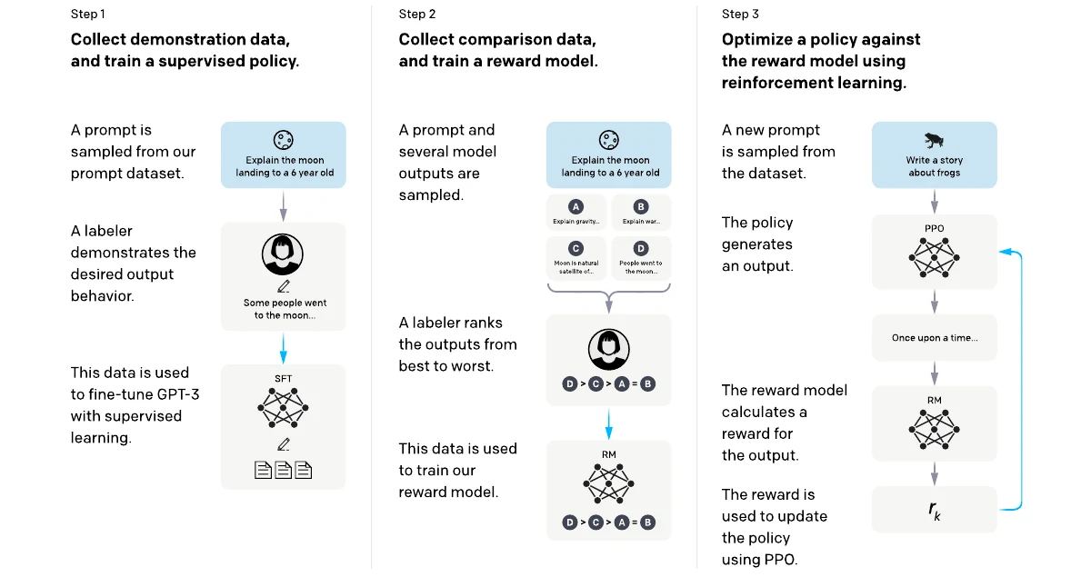
Placing this process in the reinforcement learning concept, the language model is the policy model, the Prompt and already-generated tokens constitute the current state, the model selecting the next token is equivalent to taking an action, and from starting to answer to generating the end token constitutes one complete trajectory.
In RLHF, the reward model usually gives an overall score after the response ends, and the reinforcement learning algorithm then determines which token selection probabilities should be increased. RLHF training usually also retains a reference model. The reference model is generally a frozen SFT model, used to constrain the policy model being trained from deviating too far from the original language capabilities.
Proximal Policy Optimization (PPO). It is a policy gradient algorithm whose core objective is to improve rewards while limiting the magnitude of each parameter update. Large models have many parameters; if the strategy changes drastically just because a batch of responses gets high scores, the model might quickly become biased toward a few reward patterns or even destroy its original language capabilities. The "proximal" in PPO emphasizes that the new strategy should update gradually near the old strategy. In large model post-training, one round of PPO usually includes two stages. The first stage is sampling: extracting a batch of inputs from the Prompt dataset, having the current policy model generate responses, and saving the probability of each token under the old policy, then the reward model gives scores. The second stage is updating: calculating advantages based on rewards and value estimates, using these samples to update the policy model and value model. After completing several small batch updates, the new strategy regenerates data.
PPO needs to compare the probabilities given by the new and old strategies for the same token. The probability ratio can be simplified as:
r_t(\theta) = \frac{\text{Probability of new strategy selecting current token}}{\text{Probability of old strategy selecting current token}}
Here, rₜ represents the calculated ratio, and θ represents the model being optimized.
When rₜ is close to 1, it indicates little difference between old and new strategies; when rₜ is significantly greater than 1, the new strategy is more inclined toward the current token; when rₜ is significantly less than 1, the new strategy has reduced its probability. Only probability change is not enough; the advantage Aₜ is also needed to judge whether this token selection is better or worse than the current average level. When the advantage is positive, the probability of this selection should be appropriately increased; when negative, it should be decreased.
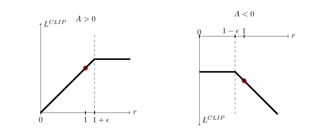
The left side of the figure above represents the situation where the advantage is positive. As the probability ratio increases from 1 to the right, the objective first increases with it; after exceeding 1+ε, the curve flattens, and continuing to increase the token's probability no longer increases the objective. The right side represents the situation where the advantage is negative. When the probability ratio drops below 1-ε, the objective also stops improving. The two curves together show that PPO allows the strategy to adjust in the correct direction but weakens the additional benefits brought by excessively large updates.
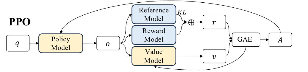
A typical large model PPO training requires maintaining several components simultaneously: the policy model is responsible for generating and accepting updates; the old strategy is a snapshot of strategy parameters during sampling, used to calculate probability ratios; the reference model is a frozen SFT model, used to calculate KL constraints; the reward model is responsible for evaluating complete responses; the value model is responsible for estimating the benefits that might be obtained at each subsequent generation position. There is a difference between the value model's estimates and actual rewards. PPO usually uses methods like GAE to organize these differences into advantages for each token. The overall PPO process is shown in the figure below. The policy model generates response o based on input q, the reward model and reference model together form reward r, the value model gives value estimate v, and then advantage A is calculated through GAE. The policy model updates based on advantages and clipping objectives, while the value model learns more accurate benefit estimates through value loss.
Group Relative Policy Optimization (GRPO). It is a variant of PPO that retains ideas like strategy sampling, probability ratio clipping, and KL constraints. The main change is that it no longer trains a separate value model but uses the relative scores of multiple responses to the same Prompt to estimate advantages. The overall GRPO framework is shown in the figure below. For the same input q, the policy model generates a group of responses o₁ to oG at once, and the reward model or rule system gives r₁ to rG respectively.
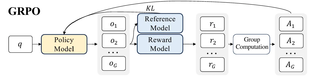
The system first calculates the mean and standard deviation of this group of rewards, then converts each response's score to relative advantage within the group. Responses with scores above the group average get positive advantages, while those below get negative advantages. For tasks where only one overall reward is given at the end of the response, tokens in the same response usually share the relative advantage obtained by that response. If process rewards are also provided, finer token-level feedback can be further formed. Subsequently, GRPO compares new and old strategy probabilities like PPO and updates the policy model through clipping objectives and KL constraints.
Compared to PPO, GRPO reduces the parameters, memory, and training overhead brought by the value model, but this doesn't mean training costs are necessarily low. Each Prompt needs to generate multiple responses, and inference sampling itself consumes significant computational resources. If all responses in the same group have the same score with standard deviation close to 0, group comparison will find it difficult to provide effective direction, and actual implementation needs to skip, smooth, or resample such data. Group size, sampling temperature, reward scale, and KL coefficient also affect training stability. For example, a math question generates four solutions, two of which are correct, one has a calculation error, and one is incomplete. The system can use answer verification rules to score them, then compare within the four results. Correct and complete responses get higher advantages, while incorrect or incomplete responses get lower advantages, and the model increases the probability of better solutions accordingly. Code tasks can also use compilation results and unit tests as rewards without necessarily first training a dedicated reward model.
Direct Preference Optimization (DPO). In its paper title, the authors clearly state that preference models might not be needed, and the large language models we build might themselves be potential preference models. This idea directly abandons separate modeling of preference models, instead starting from the original model and adding a loss function specifically designed for preference models, enabling further improvement in optimizing model generation results. DPO directly trains language models using already-collected preferred and non-preferred responses, without needing to explicitly train a reward model or run online reinforcement learning loops like PPO or GRPO.
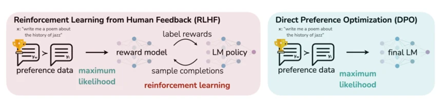
The figure above compares the classical RLHF pipeline with DPO. Preference data is first used to train the reward model, then the policy model generates new responses, which undergo reinforcement learning based on the reward model's scores. In the DPO pipeline, preference data goes directly into language model training. Both pipelines start from the superiority relationship between responses, but the training steps and resource requirements differ. The overall DPO process requires only two stages:
The first stage involves constructing positive and negative samples from preference data. Compared to the previous fine-tuning stage's sample construction method, this step changes the original "input-output" dataset to "input-accepted response-negative response." This sample training method is not new; it actually originated from contrastive learning in the image domain. Researchers in contrastive learning found that when models learn positive and negative examples simultaneously, the model can converge quickly and overall performance can be further improved.
The second stage is based on the designed loss function, using contrastive learning methods and maximum likelihood to optimize the original generation model's parameters. This design eliminates the original preference reward model and the entire reinforcement learning process training. While efficiency is improved, accuracy and stability are also significantly improved compared to PPO. Through second-stage optimization adjustments, model parameters are continuously optimized in the direction of moving closer to positive examples and away from negative examples, ultimately achieving preference alignment of model generation toward positive example content.
DPO's training form is similar to regular SFT. Training data already contains Prompts, preferred responses, and non-preferred responses. The model doesn't need to regenerate candidates at each step, nor does it need to run the reward model and value model simultaneously. Therefore, it belongs to offline preference optimization with fewer components, usually lower memory and engineering complexity than PPO. This simplification does not eliminate the requirements for data quality. DPO can only learn the differences that already appear in preference data. If the preferred response itself has factual errors, the non-preferred response is too inferior, or the data mainly comes from a generation distribution very different from the current model, the model might learn superficial styles rather than target capabilities. DPO also won't continuously explore new responses like online reinforcement learning, then obtain feedback on newly emerged problems.
The previous sections have introduced the basic principles and training methods of RLHF, PPO, GRPO, and DPO separately. To understand the relationships between them more clearly, we can compare them from several dimensions including method positioning, whether online response generation is needed during training, and whether they depend on reward models and value models. Through this horizontal comparison, we can more intuitively see the main differences between different post-training methods in implementation paths, training costs, and applicable methods. The table below shows the model comparison.
Concept | Category | Generates new responses during training? | Requires explicit reward model? | Requires value model? | Key characteristics |
RLHF | Feedback and reinforcement learning framework | Usually yes | Classical pipeline requires it | Depends on optimization algorithm used | Defines how human feedback, rewards, and policy updates connect |
PPO | Online reinforcement learning algorithm | Yes | Usually required in classical RLHF | Yes | Stabilizes policy updates through value estimation and probability ratio clipping |
GRPO | Online reinforcement learning algorithm | Yes, typically generates a group of responses per Prompt | Can use reward model or rule rewards | No | Uses group-relative rewards to estimate advantages |
DPO | Offline preference optimization | Usually no online generation | No separate training needed | No | Directly increases the probability of preferred responses relative to non-preferred ones |
Overall, while RLHF, PPO, GRPO, and DPO are all related to large model preference alignment, they don't solve exactly the same problems. RLHF is more of a complete feedback and reinforcement learning framework, PPO and GRPO are online reinforcement learning algorithms used to update policy models within this type of framework, while DPO directly uses existing preference data to complete offline optimization. From the training mechanism perspective, PPO depends on reward models and value models, with a more complete overall engineering pipeline, but also higher training costs and implementation complexity; GRPO estimates advantages through group-relative rewards, eliminating the value model, and is more suitable for tasks with verifiable rewards, answer checking, and other clear feedback; DPO does not need online response generation or separate training of reward models and value models, so implementation is relatively simple and is suitable as a low-cost alignment solution when preference data is sufficient.
In practical applications, method selection should start from the model's current lack of capabilities rather than simply following a certain training algorithm. When the model cannot stably complete tasks, basic capabilities should be established through SFT first; when the model can complete tasks but response quality and preference selection are unstable, DPO, PPO, or GRPO can be further adopted. When high-quality preference data is available and quick first-round alignment is desired, DPO can be prioritized; when tasks have verifiable rewards and the model is expected to actively explore better solutions, GRPO can be considered; when mature reward models, value models, and reinforcement learning infrastructure are available and fine-grained online policy update control is needed, PPO can be adopted. Regardless of which method is ultimately chosen, effectiveness cannot be judged solely by training loss, reward scores, or preference win rates; instead, continuous evaluation of the model's accuracy, task completion, safety, business boundaries, and general capabilities in real tasks is needed. The ultimate goal of post-training is not to obtain higher rewards, but to make the model more stable and reliable in completing target tasks in real usage environments.
The previous sections introduced the basic principles of preference alignment and reinforcement learning. Below we use ms-swift to complete two specific experiments. The first experiment uses Chinese preference data for DPO training, observing how the model's preference for preferred and non-preferred responses changes. The second experiment uses math problems for GRPO training, having the model generate candidate responses and then obtaining rewards based on answers and format. Both experiments use Qwen2.5-0.5B-Instruct, which already has instruction-following capability, as the initial model, each training an independent LoRA adapter.
This experiment is completed in ModelScope Notebook's single-GPU environment, with models and raw data files downloaded from ModelScope community. The configurations for the two experiments are as follows:
Item | DPO Chinese Preference Alignment | GRPO Math Answer Optimization |
Initial model | Qwen/Qwen2.5-0.5B-Instruct | Same Qwen2.5-0.5B-Instruct weights |
Dataset | AI-ModelScope/hh_rlhf_cn | AI-ModelScope/gsm8k |
Subset used | helpful_base_cn | main |
Training set | 256 preference pairs | 128 problems |
Validation set | 32 preference pairs | 16 problems |
Test set | 32 preference pairs | Official test file's 1319 problems |
Training method | LoRA, 20 optimizer update steps | LoRA, 10 optimizer update steps |
Training feedback | Preferred and non-preferred responses given in data | Rewards calculated by rules after model generates responses |
The training scale here is small, mainly for demonstrating the complete process. Training steps represent the number of optimizer parameter updates, not training epochs, and do not indicate that all training data has been used. This practical section only used a small portion of data with fewer iteration steps, and the experiment is for reference only.
After opening the accompanying Notebook, first check whether the GPU is available and the software versions actually used by the current kernel.
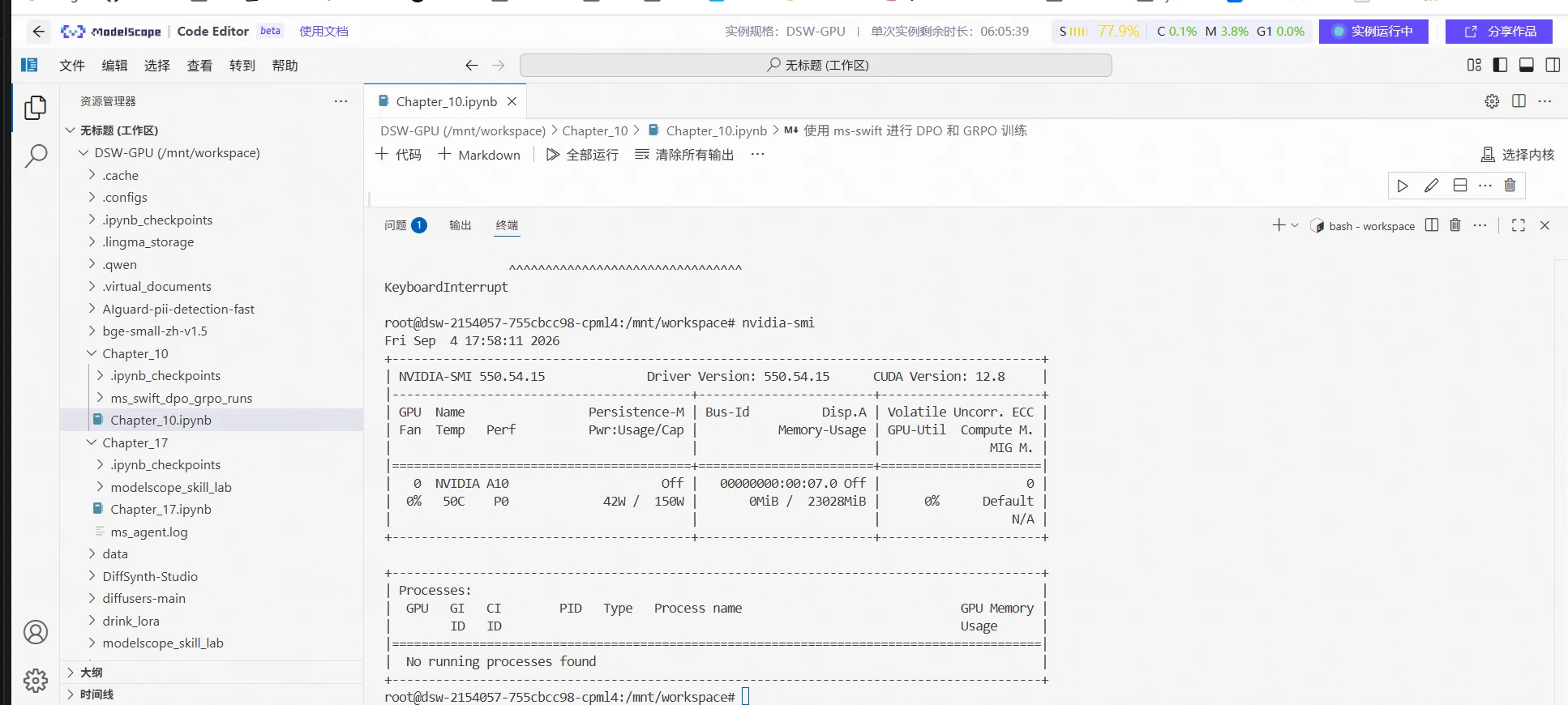
The common preparation section will establish cache and experiment directories. The core model configuration code is as follows:
MODEL_ID = "Qwen/Qwen2.5-0.5B-Instruct"
MODEL_REVISION = "master"
DPO_DATA_ID = "AI-ModelScope/hh_rlhf_cn"
GRPO_DATA_ID = "AI-ModelScope/gsm8k"
SEED = 42

MODEL_DIR = Path(snapshot_download(
    MODEL_ID,
    revision=MODEL_REVISION,
    cache_dir=str(CACHE_DIR / "models"),
    allow_file_pattern=[
        "*.json", "*.safetensors", "*.txt", "*.model", "*.tiktoken"
    ],
).resolve())
Here, snapshot_download comes from ModelScope, and CACHE_DIR is established by the common preparation code. After downloading, both training and inference use the local model snapshot pointed to by MODEL_DIR. This practical content will be saved in the ms_swift_dpo_grpo_runs/ directory. When readers re-run, the program will generate new experiment numbers, and the subsequent RUN_DIR should use your own running directory.
DPO needs two candidate responses under the same context. The experiment uses the helpful_base_cn subset of the Chinese HH-RLHF dataset, where context saves conversation history, chosen saves the preferred response, and rejected saves the non-preferred response. The preferred and non-preferred here come from dataset labels, not indicating that facts in the responses have been verified item by item.
The preference sample structure used by ms-swift is as follows. Below only shows field relationships; actual content is read from the dataset:
{
  "messages": [
    {"role": "user", "content": "Same question"},
    {"role": "assistant", "content": "Preferred response"}
  ],
  "rejected_response": "Non-preferred response"
}
Compared to the SFT samples from the earlier ms-swift quick start, rejected_response is added here. The last assistant message in messages saves the preferred response, and the non-preferred response is placed in a separate field. Historical assistant messages in multi-turn conversations still belong to context and should not be mistakenly treated as this comparison's responses. The conversion function in the Notebook is as follows:
def convert_dpo(row):
    role_map = {
        "human": "user", "user": "user",
        "assistant": "assistant", "system": "system"
    }
    context = [
        {"role": role_map[m["role"]], "content": m["text"].strip()}
        for m in row["context"]
    ]
    chosen = row["chosen"]["text"].strip()
    rejected = row["rejected"]["text"].strip()

    assert context and context[-1]["role"] == "user"
    assert chosen and rejected and chosen != rejected
    assert all(m["content"] for m in context)
    if context[0]["role"] != "system":
        context.insert(0, {"role": "system", "content": GENERAL_SYSTEM})

    return {
        "messages": context + [{"role": "assistant", "content": chosen}],
        "rejected_response": rejected,
    }
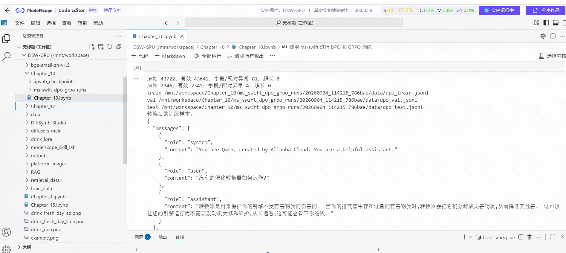
This time, the lengths of the preferred and non-preferred responses after concatenation with context are calculated separately, and only samples where neither exceeds 1024 tokens are retained. When exceeding the limit, the entire pair of data is discarded to avoid truncation that might delete the key content determining response quality. Then, deduplication is performed by context, and 256 training data and 32 validation data are split from the original training source. The processed files are dpo_train.jsonl, dpo_val.jsonl, and dpo_test.jsonl, saved in the data folder of this run directory. The three files serve different purposes: the training set is for updating parameters, the validation set is for observing the training process, and the test set is for independent comparison after training. The relevant execution results are shown in the figure below.
Before training, first use the initial model to record performance on the test set. The dpo_evaluate() in the Notebook calculates the log probabilities of responses for 32 fixed candidate pairs and generates responses for 4 of them for comparison after training:
def dpo_evaluate(adapter=None):
    def action(model):
        rows = []
        for index, row in enumerate(dpo_test):
            context = row["messages"][:-1]
            lp_chosen = response_logp(model, context, row["messages"][-1]["content"])
            lp_rejected = response_logp(model, context, row["rejected_response"])
            rows.append({"sample_id": index, "chosen_logp": lp_chosen,
                         "rejected_logp": lp_rejected, "gap": lp_chosen - lp_rejected})
        generations = [{"sample_id": i, "context": dpo_test[i]["messages"][:-1],
                        "response": generate_one(model, dpo_test[i]["messages"][:-1])}
                       for i in range(min(4, len(dpo_test)))]
        return rows, generations
    return with_local_model(action, adapter)

dpo_before, dpo_before_text = dpo_evaluate()
The relevant steps for starting DPO training are as follows:
The two experiments reuse common configurations through common_options(), including local model path, Qwen chat template, random seed, bfloat16 precision, and LoRA settings. LoRA rank is 8, alpha is 16, and the target modules are all-linear. Below is the complete DPO experiment configuration; the common function needs to be run first in the accompanying Notebook. The common_options() function merges common parameters with this experiment's parameters. train_swift converts these parameters to command-line form and calls swift.cli.rlhf through the current kernel's Python for model training.
DPO_OUTPUT = RUN_DIR / "dpo"
DPO_BETA = 0.1
dpo_options = common_options() | {
    "rlhf_type": "dpo", "loss_type": "sigmoid", "beta": DPO_BETA,
    "dataset": str(DPO_PATHS["train"]),
    "val_dataset": str(DPO_PATHS["val"]),
    "output_dir": str(DPO_OUTPUT), "max_length": 1024,
    "truncation_strategy": "delete", "max_steps": 20,
    "learning_rate": 5e-5, "lr_scheduler_type": "cosine",
    "warmup_ratio": 0.1,
    "per_device_train_batch_size": 1,
    "per_device_eval_batch_size": 1,
    "gradient_accumulation_steps": 8,
    "eval_strategy": "steps", "eval_steps": 10,
    "save_strategy": "steps", "save_steps": 10,
}
train_swift(dpo_options, RUN_DIR / "dpo_train.log")
DPO_ADAPTER = latest_adapter(DPO_OUTPUT)
The meanings of the main parameters are as follows:
Parameter | Value in this experiment | Purpose |
rlhf_type / loss_type | dpo / sigmoid | Uses standard sigmoid-form DPO objective |
beta | 0.1 | Controls the scale relative to reference strategy in DPO objective |
learning_rate | 5e-5 | Controls the magnitude of each parameter update |
max_length | 1024 | Limits the total length of context and candidate responses |
per_device_train_batch_size | 1 | Single GPU processes 1 preference pair per training micro-batch |
gradient_accumulation_steps | 8 | Accumulates 8 micro-batches before updating parameters once |
max_steps | 20 | Ends training after 20 optimizer updates |
eval_steps / save_steps | 10 / 10 | Validates and saves checkpoints every 10 steps |
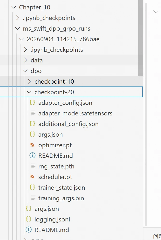
After training starts, ms-swift will output loss, implicit rewards, validation metrics, and checkpoint save locations. After this training completes, the model will be saved in the dpo/checkpoint directory. The model training and saving results are shown in the figure below.
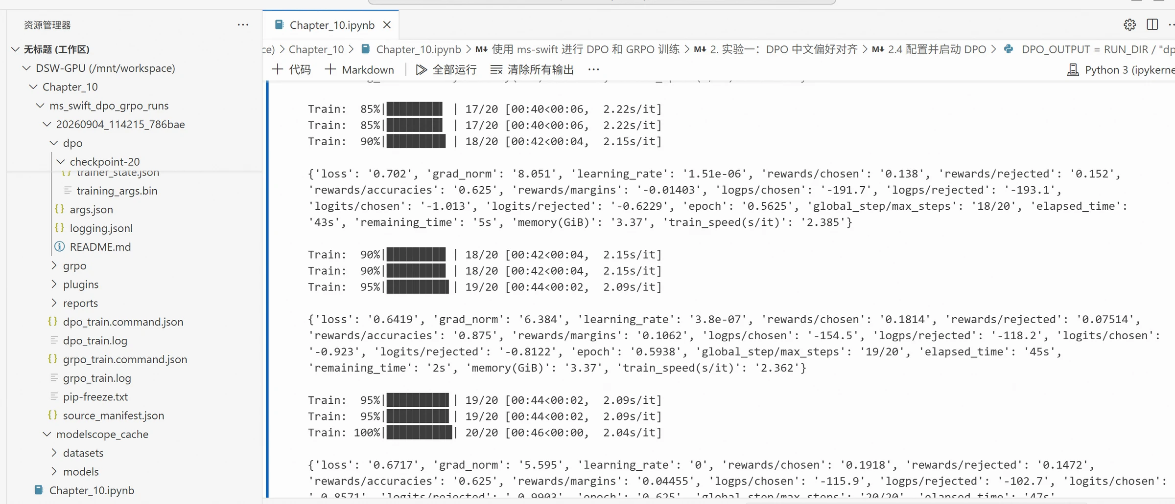
The rewards/chosen and rewards/rejected in the logs are implicit rewards calculated based on the log probability difference between the policy and reference strategy, not scores given by some external reward model for response quality. rewards/accuracies represents the proportion where implicit reward ranking matches preference labels and should not be directly understood as the accuracy of model-generated responses. The relevant log execution results are shown in the figure below.
After loading the DPO adapter, evaluate again using the same test data. Keep the system prompt, chat template, and generation parameters consistent during comparison to avoid treating prompt changes or decoding method changes as training effects.
dpo_after, dpo_after_text = dpo_evaluate(DPO_ADAPTER)
before_df = pd.DataFrame(dpo_before).set_index("sample_id")
after_df = pd.DataFrame(dpo_after).set_index("sample_id")

comparison = pd.DataFrame({
    "before_gap": before_df["gap"],
    "after_gap": after_df["gap"],
    "relative_dpo_margin": DPO_BETA * (
        after_df["gap"] - before_df["gap"]
    ),
})
Here, gap equals the preferred response's sequence log probability minus the non-preferred response's sequence log probability. When gap is greater than 0, it indicates the current model has higher sequence probability for the given preferred response. The proportion of test samples satisfying this condition gives the pair_preference_rate.
The test results are shown in the figure below:
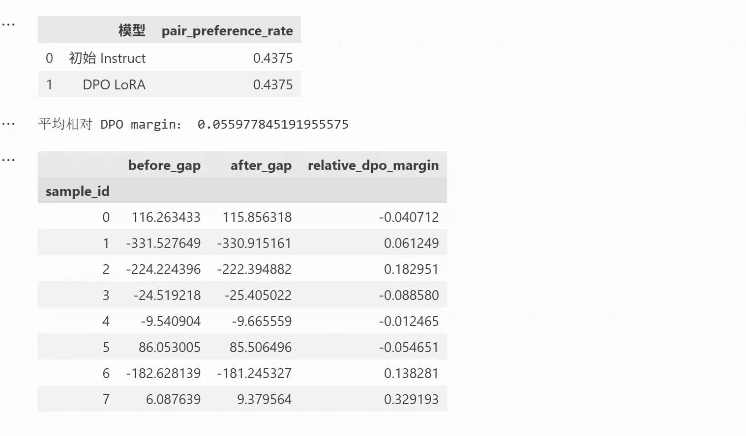
Due to the small number of training epochs, some samples' differences can increase but still haven't changed from negative to positive. Some samples improved while others regressed. Therefore, a positive average relative margin doesn't necessarily increase the proportion of preferred responses winning. In this experiment, that proportion remained at 43.75% before and after training. Taking a test sample where a user asks about home network signal as an example:
User: What methods can I use to strengthen my home network signal? My laptop has trouble connecting to the network router!
The initial model's response contained the following, excerpted from the original:
1. **Use a wireless router**: If you have multiple devices in your home that need to access the internet, consider installing a wireless router. This will allow you to connect to the internet via Wi-Fi.
The DPO-trained response contained:
3. **Restart the router**: Sometimes, a simple restart can resolve some network connection issues. Please follow the router's instructions.
From the full output, the initial response suggested changing or adding devices more frequently, while after training, the response organized more around network settings, drivers, and restart operations, indicating that training changed the generation content. This DPO training changed the relative probabilities of some fixed candidates and some generated responses, but due to the limited training steps and data, readers can experiment with larger data and more training epochs.
DPO uses two responses already given in the data, while GRPO needs the model to generate candidate responses during training, which are then evaluated by the reward function. This experiment uses GSM8K math application problems, using the final number and output format as automatically checkable feedback, without training a separate reward model.
The original GSM8K dataset contains question and answer fields. The answer field contains both the solution process and the final number after ####. During data conversion, only the question is given to the model, and the final number is extracted to the solution field. The relevant code is as follows:
def convert_grpo(row):
    question = row["question"].strip()
    original_answer = row["answer"].strip()
    assert question and "####" in original_answer
    answer = parse_numeric(original_answer.rsplit("####", 1)[-1])
    assert answer is not None
    return {
        "messages": [
            {"role": "system", "content": MATH_SYSTEM},
            {"role": "user", "content": question},
        ],
        "solution": str(answer),
    }
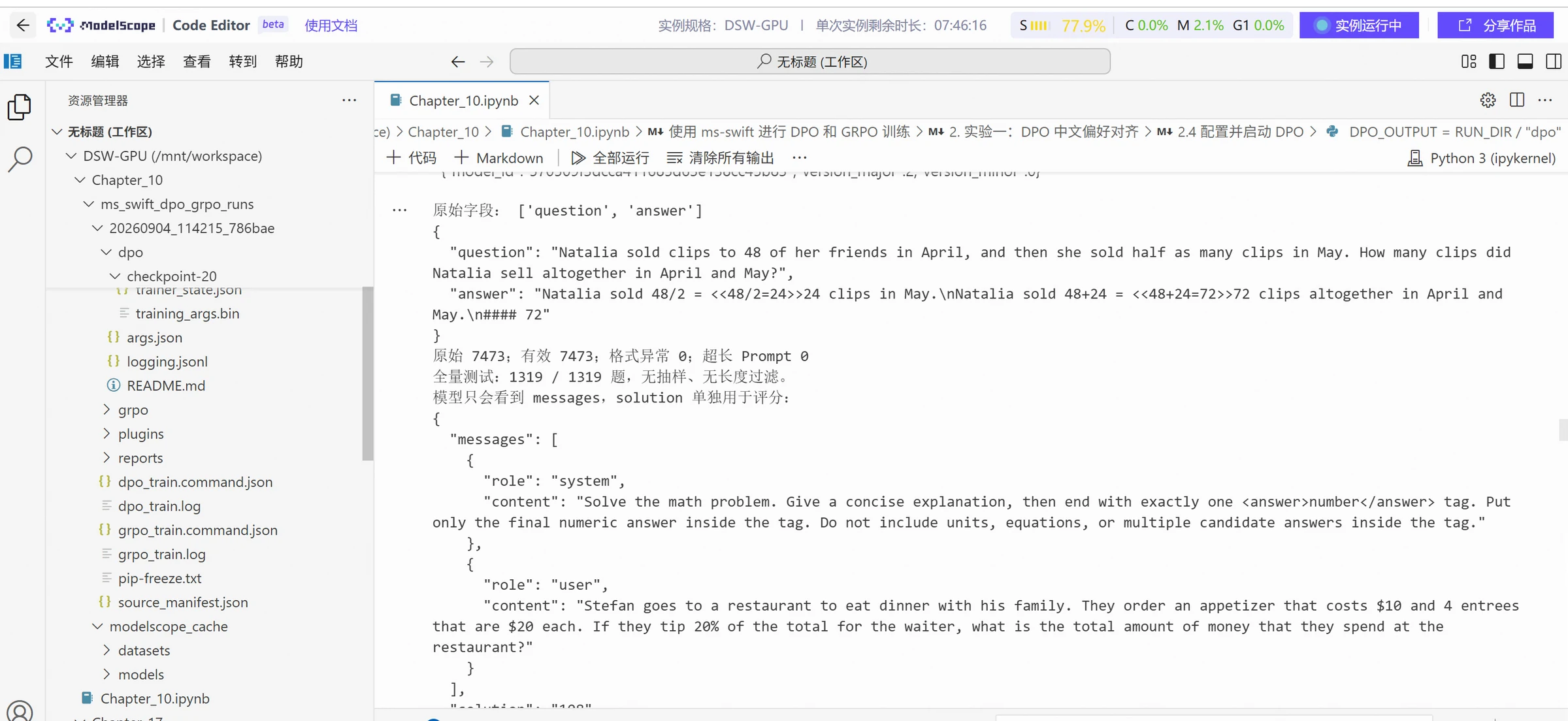
The converted messages has no standard solution process and no assistant response for the model to imitate. The solution is passed to the reward function as an additional data column and is not concatenated into the Prompt. This way, during training, the model needs to generate its own answer, and the scoring program compares it with the standard answer. This time, 128 training problems and 16 validation problems are cleaned, deduplicated, and split from the original training source. Training and validation Prompts have a length limit of 512 tokens. The test uses all 1319 problems from the official test file, preserving the original order, not deleting problems based on training length thresholds, and checking for overlap with training and validation data. The relevant execution results are shown below:
The total reward for this experiment is:
Total reward = Correctness reward + 0.1 × Format reward
The correctness reward requires the model output to match the specified label format, and the number in the label equals solution, which is 1 when satisfied and 0 otherwise. The format reward only checks whether the label is unique, located at the end of the response, and whether the content can be parsed as a number, which is 1 when satisfied and 0 otherwise. The relevant code is as follows:
def extract_answer(completion):
    if not isinstance(completion, str):
        return None
    if completion.count("<answer>") != 1 or completion.count("</answer>") != 1:
        return None
    match = re.search(r"<answer>\s*([^<>]+?)\s*</answer>\s*\Z", completion)
    return parse_numeric(match.group(1) if match else None)

class Chapter10Accuracy(ORM):
    def __call__(self, completions, solution, **kwargs):
        if len(completions) != len(solution):
            raise ValueError("Candidate responses and solution count mismatch.")
        rewards = []
        for text, gold in zip(completions, solution):
            expected = parse_numeric(gold)
            if expected is None:
                raise ValueError(f"Invalid standard answer format: {gold!r}")
            predicted = extract_answer(text)
            rewards.append(float(predicted is not None and predicted == expected))
        return rewards

class Chapter10Format(ORM):
    def __call__(self, completions, **kwargs):
        return [float(extract_answer(text) is not None) for text in completions]
Here, completions is a group of model-generated responses, and solution is the corresponding standard answer passed by the trainer. extract_answer first checks the label count, then confirms the label is at the end of the response, and finally extracts the number. This reward only checks the final result, not the solution process. Even without explanations, the model can receive full reward as long as it outputs the correct answer label. The "brief explanation" in the system prompt is not written into the scoring conditions, so high scores should not be understood as the model having learned complete and reliable reasoning.
The reward class also needs to be registered. The reward plugins used by this trainer are:
orms["chapter10_accuracy"] = Chapter10Accuracy
orms["chapter10_format"] = Chapter10Format
The Notebook saves the complete plugin as plugins/chapter10_rewards.py. Later, external_plugins specifies the file path, and reward_funcs specifies the above registration names. The plugin should contain its own imports and helper functions because it is loaded independently in the training subprocess. Registration methods can refer to the ms-swift 4.4.2 official reward plugin example.
The following are the reward calculation results for some of the results:
Model output | Standard answer | Correctness reward | Format reward | Total reward |
| 12 | 1 | 1 | 1.1 |
| 12 | 1 | 1 | 1.1 |
| 12 | 0 | 1 | 0.1 |
| 12 | 0 | 0 | 0 |
| 12 | 0 | 0 | 0 |
| 12 | 0 | 0 | 0 |
According to the reward function calculation method used this time, even though the plain text The answer is 12. contains the correct number, it doesn't meet the format requirements, so the strict correctness reward is still 0. Multiple answer labels also won't pass the check, preventing the model from gaining rewards by enumerating answers.
After completing data and reward function preparation, complete the relevant experiment setup and training tasks.
This experiment generates 4 candidate responses for each problem, with generation batch also set to 4, so one generation batch corresponds to 4 candidates for one problem. Subsequently, each training micro-batch processes 1 candidate, accumulating 4 micro-batches before updating parameters once.
The following is the GRPO experiment configuration for this time. GRPO_PATHS, PLUGIN_PATH, and related configurations and content.
GRPO_OUTPUT = RUN_DIR / "grpo"
grpo_options = common_options() | {
    "rlhf_type": "grpo", "loss_type": "grpo",
    "dataset": str(GRPO_PATHS["train"]),
    "val_dataset": str(GRPO_PATHS["val"]),
    "output_dir": str(GRPO_OUTPUT),
    "external_plugins": str(PLUGIN_PATH),
    "reward_funcs": ["chapter10_accuracy", "chapter10_format"],
    "reward_weights": [1.0, 0.1], "remove_unused_columns": False,
    "num_generations": 4, "generation_batch_size": 4,
    "per_device_train_batch_size": 1,
    "gradient_accumulation_steps": 4,
    "per_device_eval_batch_size": 4, "num_generations_eval": 4,
    "max_length": 512, "max_completion_length": 256,
    "truncation_strategy": "left",
    "max_steps": 10, "learning_rate": 1e-5,
    "lr_scheduler_type": "constant", "warmup_ratio": 0.0,
    "beta": 0.04, "num_iterations": 1,
    "temperature": 0.9, "top_p": 0.95,
    "use_vllm": False, "log_completions": True,
    "eval_strategy": "steps", "eval_steps": 5,
    "save_strategy": "steps", "save_steps": 5,
}
train_swift(grpo_options, RUN_DIR / "grpo_train.log")
GRPO_ADAPTER = latest_adapter(GRPO_OUTPUT)
The group size and generation batch need to be configured together. The generation batch must be divisible by the group size, and also divisible by the product of single-GPU training micro-batch and the number of GPU processes. This time it's single GPU single process, with generation batch 4, group size 4, and training micro-batch 1 satisfying these conditions; during validation, batch and group size are also both 4. If adjusting the group size, verify the generation batch, training gradient accumulation, and validation configuration together. This training completed 10 steps and saved grpo/checkpoint-10.
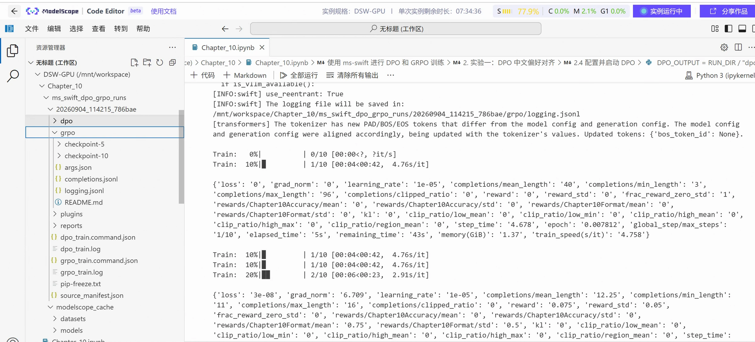
The GRPO training loss is not math problem accuracy. When observing training, look at total reward, reward sub-items, and within-group differences together. The reward in the logs indicates the currently aggregated reward, reward_std is used to observe within-group reward differences, and frac_reward_zero_std indicates the proportion of groups where within-group reward standard deviation is zero. The relevant training statistics visualization results are shown in the figure below:
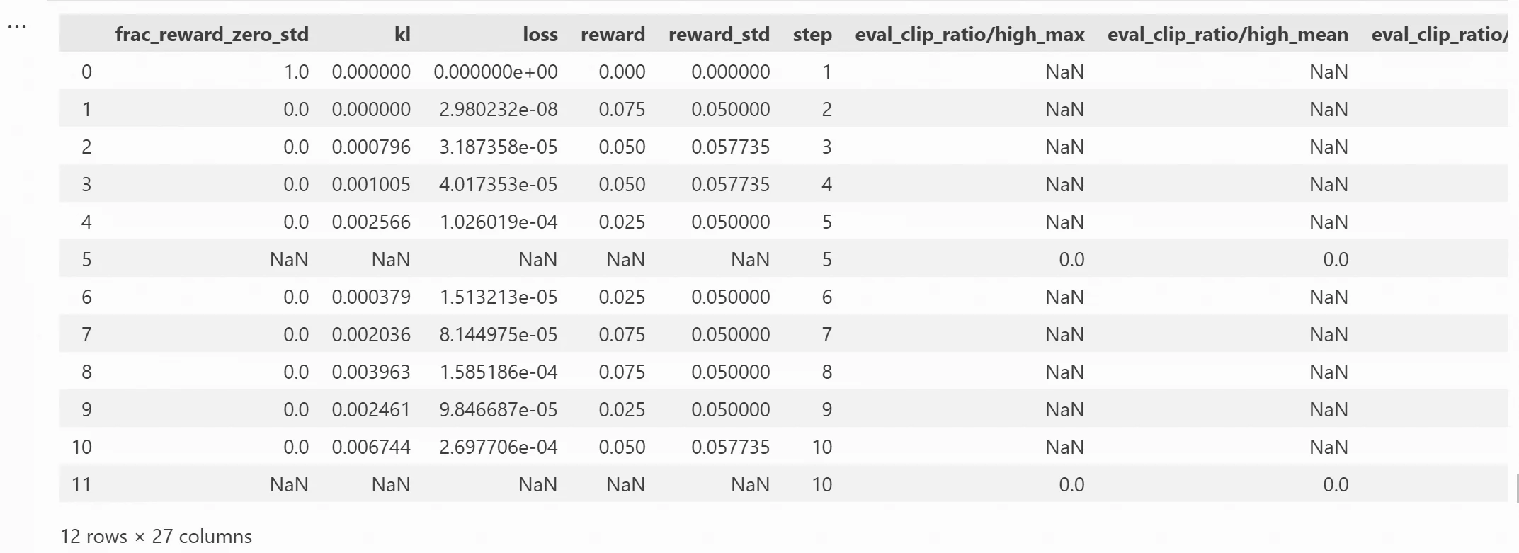
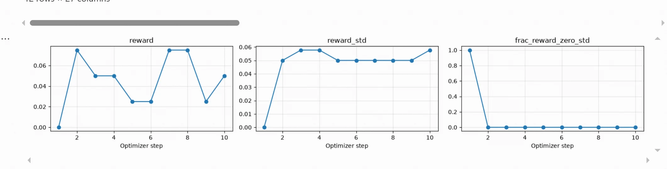
From the figure, it can be seen that training started showing non-zero within-group reward differences from step 2, with same-score proportion dropping to 0, indicating the reward function can already distinguish different candidate responses and provide effective optimization signals for GRPO. Only 10 training steps were performed this time, with sparse correctness rewards and math answer accuracy not yet improved. Subsequently, training epochs can be increased to let the model encounter more problems and candidate responses, combined with validation set observation for more obvious training effects.
Training logs reflect the candidates sampled during training, and ultimately an independent test set is needed to compare model performance. Each problem only generates one response, not multiple random samplings to select the best answer.
Initial results were saved by grpo_evaluate() before training. After training, the GRPO adapter is passed in, and then results on the same problems are summarized below. The evaluation and summary code is excerpted; the Notebook also checks whether sample numbers, problems, and standard answers correspond one-to-one.
grpo_after = grpo_evaluate(GRPO_ADAPTER)
grpo_summary = pd.DataFrame([
    {
        "Model": name,
        "Strict answer accuracy": np.mean([r["correct"] for r in rows]),
        "Correct problems": int(sum(r["correct"] for r in rows)),
        "Valid format ratio": np.mean([r["format_ok"] for r in rows]),
        "Format-passing problems": int(sum(r["format_ok"] for r in rows)),
        "Average total reward": np.mean([r["total_reward"] for r in rows]),
        "Test problems": len(rows),
    }
    for name, rows in [
        ("Initial Instruct", grpo_before), ("GRPO LoRA", grpo_after)
    ]
])
display(grpo_summary)
The full evaluation results are as follows:

Combined with the above full evaluation results, the model's valid format ratio increased from 89.16% to 94.24%, reflecting the role of this training in standardizing output format. Subsequent experiments and training can further adjust problem difficulty or reward design to enable subsequent results to receive more sufficient answer correctness feedback.
All experimental data and code for this chapter can be referenced at: https://modelscope.cn/gallery/liucong/8a5fefc5-6f90-42df-9a09-bc9781ed3da8